
Data Analysis Using SPSS: From a Codebook to a Reproducible Workflow
A polished output file does not establish a correct workflow. Others must know how data were coded, checked and transformed before model estimation.
A reproducible SPSS workflow preserves unchanged raw data, defines missingness clearly, performs consequential steps through syntax and retains a trace from data to report. Syntax supports reviewing command order and rerunning analyses after data change (IBM, n.d.-a; Wilson et al., 2017).
A reproducible analysis workflow
- Codebook
Variable names, coding and missingness
- Preparation
Record data-cleaning steps
- Analysis
Keep configuration and analysis code
- Records
Save results and software versions
Conceptual diagram. Preserve original data and a change trail for verification.
Source: Lê Minh · Conceptual illustration, not software output.1. Define outputs before opening SPSS
Data processing means more than editing a few Data View cells. The aim is an analysis dataset with clear provenance, a rerunnable command file and results matching the research question.
Before importing data, document dependent, explanatory and control variables, score scales and exclusion rules in the codebook. Subsequent auditing becomes nearly impossible if these decisions exist only in the analyst's memory.
| Output | Required content | Verification |
|---|---|---|
| Codebook | Names, labels, value codes, missingness and measurement levels | Compare with questionnaire and Variable View |
| Analysis data | Cleaned and derived variables | Recreate from raw data using syntax |
| Syntax | Import, checks, transformations and analysis | Run from the start in a fresh session |
| Output | Tables, plots, warnings and models | Match syntax and data version |
| Decision log | Reasons for recoding, excluding cases or changing models | Include date, analyst and supporting rationale |
2. Organize folders and protect raw data
Keep raw data read-only. All edits should generate derived data. This follows reproducible-research principles separating data, code and results (Wilson et al., 2017).
Use stable folder and filenames. Avoid names such as final, final2 or final_moi, which do not identify which file produced the thesis results.
| Path | Role |
|---|---|
| data/raw/ | Original received files, unchanged |
| data/derived/ | .sav files generated through syntax |
| syntax/ | .sps files ordered 01, 02, 03 |
| output/ | .spv files and PDF exports |
| docs/ | Codebook, decision log and README |
When finding an incorrect value, encode the correction rule in syntax and save a derived file. This preserves the audit trail.
3. Turn the questionnaire into a codebook
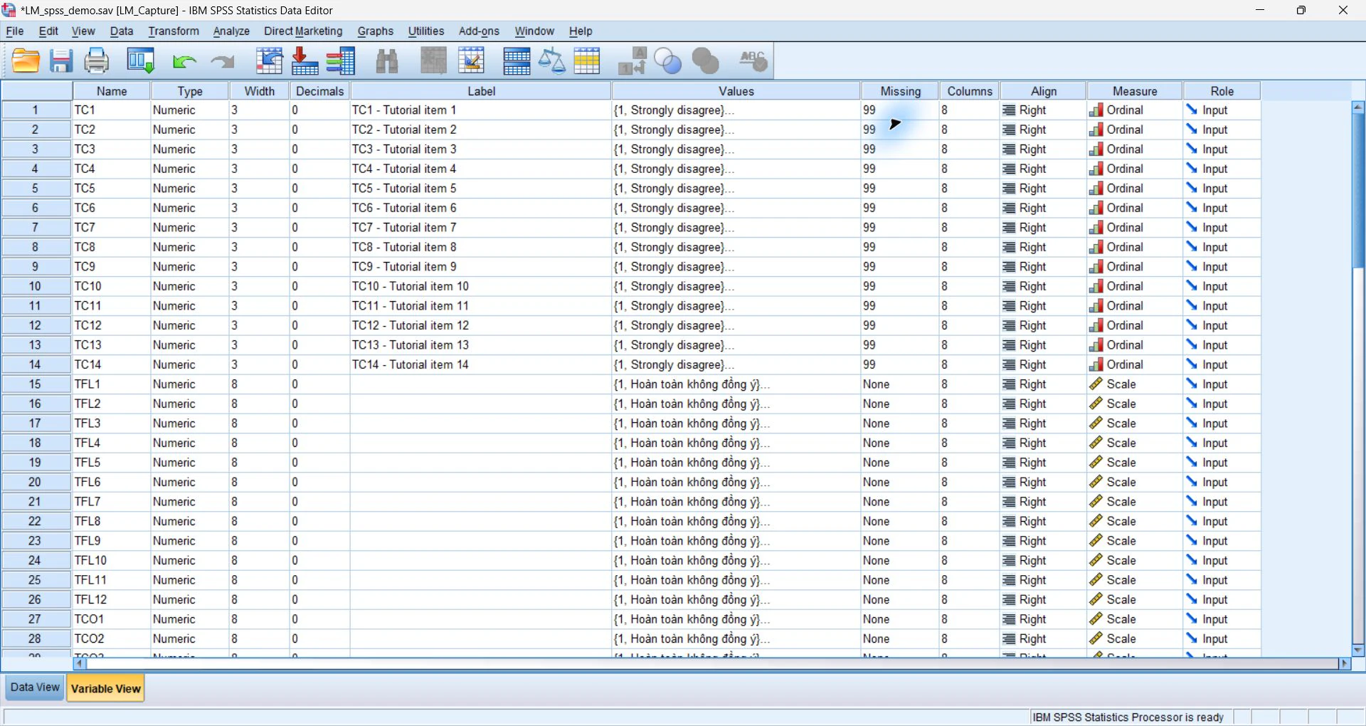
Variable View is the codebook's technical representation, but maintain an independently readable codebook table. Each row describes a variable. Minimum columns are variable name, question, data type, value labels, missing codes, valid range and analytical role.
Distinguish system-missing from user-missing. System-missing occurs when SPSS has no numeric value. User-missing is an intentional code, such as 99 for not applicable. SPSS handles it correctly only after the code is declared (IBM, n.d.-b).
| Variable | Label | Valid codes | Missing | Measurement level |
|---|---|---|---|---|
| id | Respondent identifier | Unique | None | Nominal |
| gender | Self-reported gender | 1, 2, 3 | 99 | Nominal |
| satisfaction1 to satisfaction4 | Four satisfaction indicators | 1 to 5 | 99 | Ordinal |
| trust1 to trust4 | Four trust indicators | 1 to 5 | 99 | Ordinal |
| outcome | Illustrative continuous outcome | As specified by design | 99 | Scale |
4. Import data and check structure
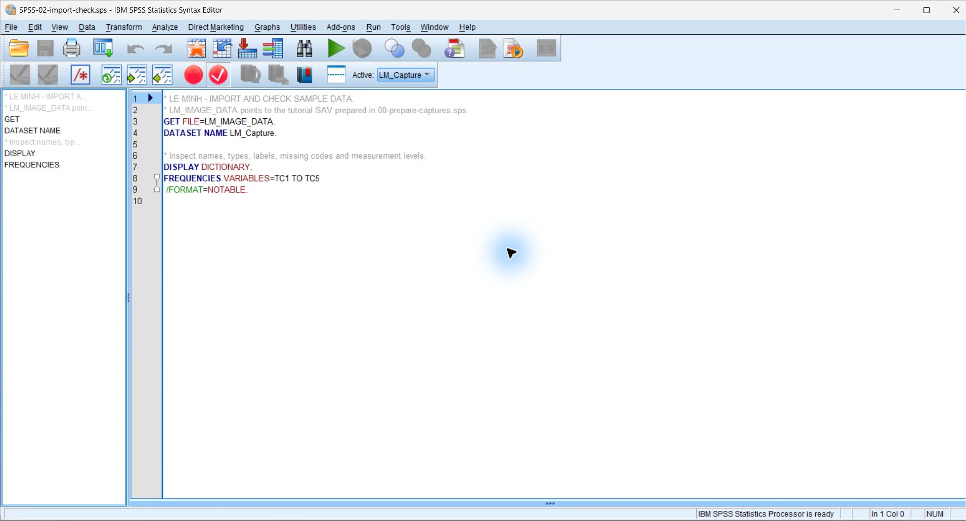
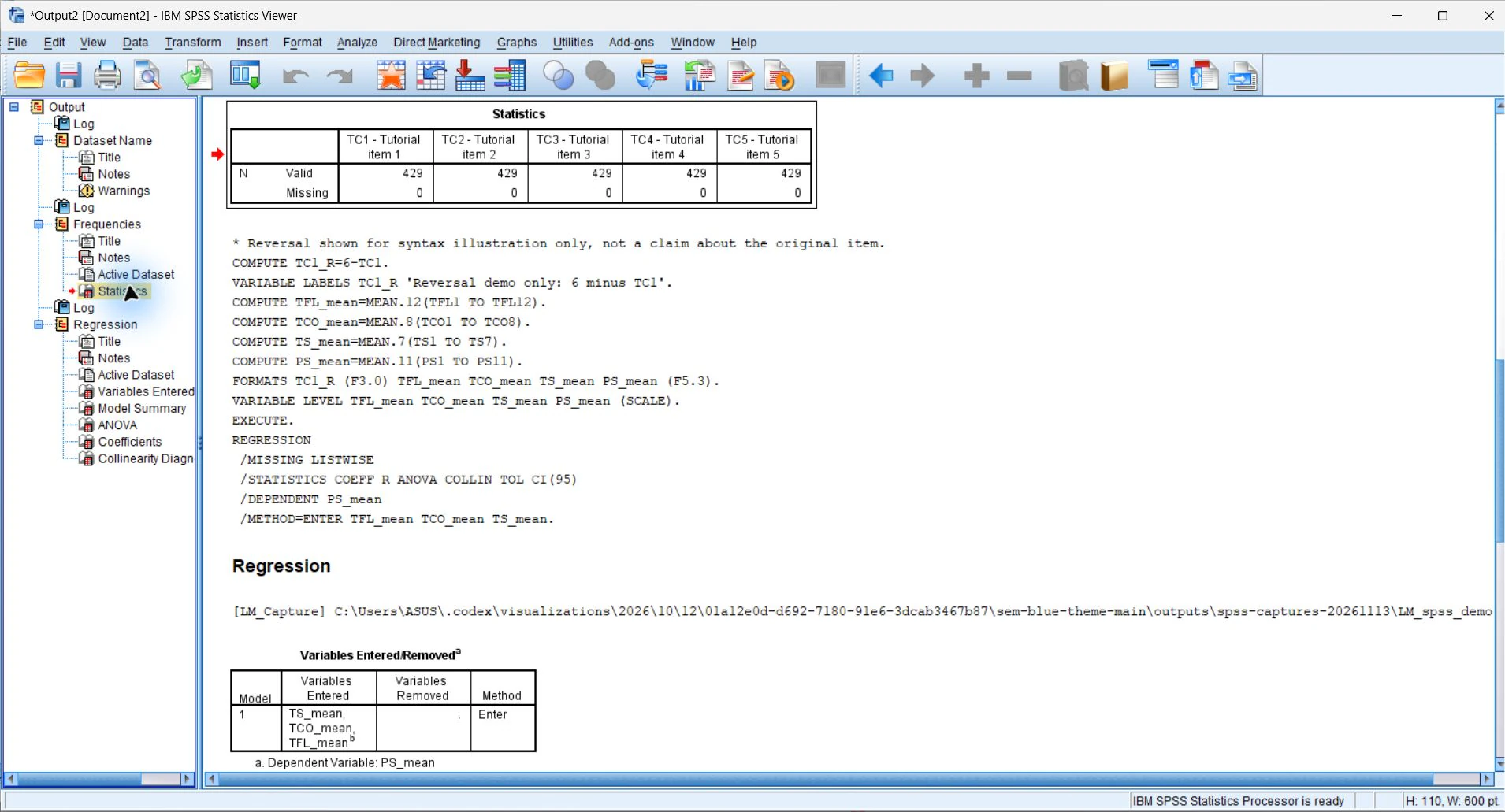
After import, check rows, variables, types, duplicate IDs and ranges before calculating scale scores. A file opening successfully does not establish correct import.
The following commands illustrate a workflow using a simulated CSV file. Adapt filenames and coding rules to the actual codebook.
GET DATA
  /TYPE=TXT
  /FILE='data/raw/survey.csv'
  /ENCODING='UTF8'
  /DELCASE=LINE
  /DELIMITERS=","
  /QUALIFIER='"'
  /ARRANGEMENT=DELIMITED
  /FIRSTCASE=2
  /IMPORTCASE=ALL.
DATASET NAME survey.

DISPLAY DICTIONARY.
FREQUENCIES VARIABLES=gender age
  satisfaction1 TO satisfaction4
  /STATISTICS=MINIMUM MAXIMUM.

SORT CASES BY id.
MATCH FILES FILE=* /BY id /FIRST=first_id.
FREQUENCIES VARIABLES=first_id.If IDs are not unique, stop and investigate before merging files or estimating models.
5. Declare and assess missing data
Define missing values before scoring. Treating code 99 as valid on a 1-to-5 scale distorts means, standard deviations and correlations.
Missing Value Analysis describes missing patterns and offers diagnostic procedures, subject to SPSS version or module availability (IBM, n.d.-c). Do not infer missingness mechanisms from a single percentage table. Examine collection design, skip logic and associations between missingness and observed variables.
MISSING VALUES gender age
  satisfaction1 TO satisfaction4
  trust1 TO trust4 outcome (99).

FREQUENCIES VARIABLES=gender age
  satisfaction1 TO satisfaction4
  trust1 TO trust4 outcome
  /ORDER=ANALYSIS.

MVA VARIABLES=satisfaction1 TO satisfaction4
trust1 TO trust4 outcome.Treatment must suit the missingness mechanism, analysis objective and estimator. Report missing rates, handling rules and sensitivity analyses when decisions could affect conclusions.
6. Create derived variables through syntax
Use RECODE with INTO to create new variables when original values must be preserved. COMPUTE generates averages, sums or interactions. After each transformation, run FREQUENCIES or DESCRIPTIVES to check ranges.
The example uses MEAN.3, creating a satisfaction score only with at least three of four valid indicators. This illustrative rule is not a universal standard. Determine the minimum from scale structure and the analysis plan.
RECODE satisfaction2 (1=5) (2=4) (3=3) (4=2) (5=1)
  INTO satisfaction2_r.
VARIABLE LABELS satisfaction2_r
  'Satisfaction item 2, reverse scored'.

COMPUTE satisfaction_mean =
  MEAN.3(satisfaction1, satisfaction2_r, satisfaction3, satisfaction4).
COMPUTE trust_mean =
  MEAN.3(trust1, trust2, trust3, trust4).
EXECUTE.

DESCRIPTIVES VARIABLES=satisfaction_mean trust_mean
  /STATISTICS=MEAN STDDEV MIN MAX.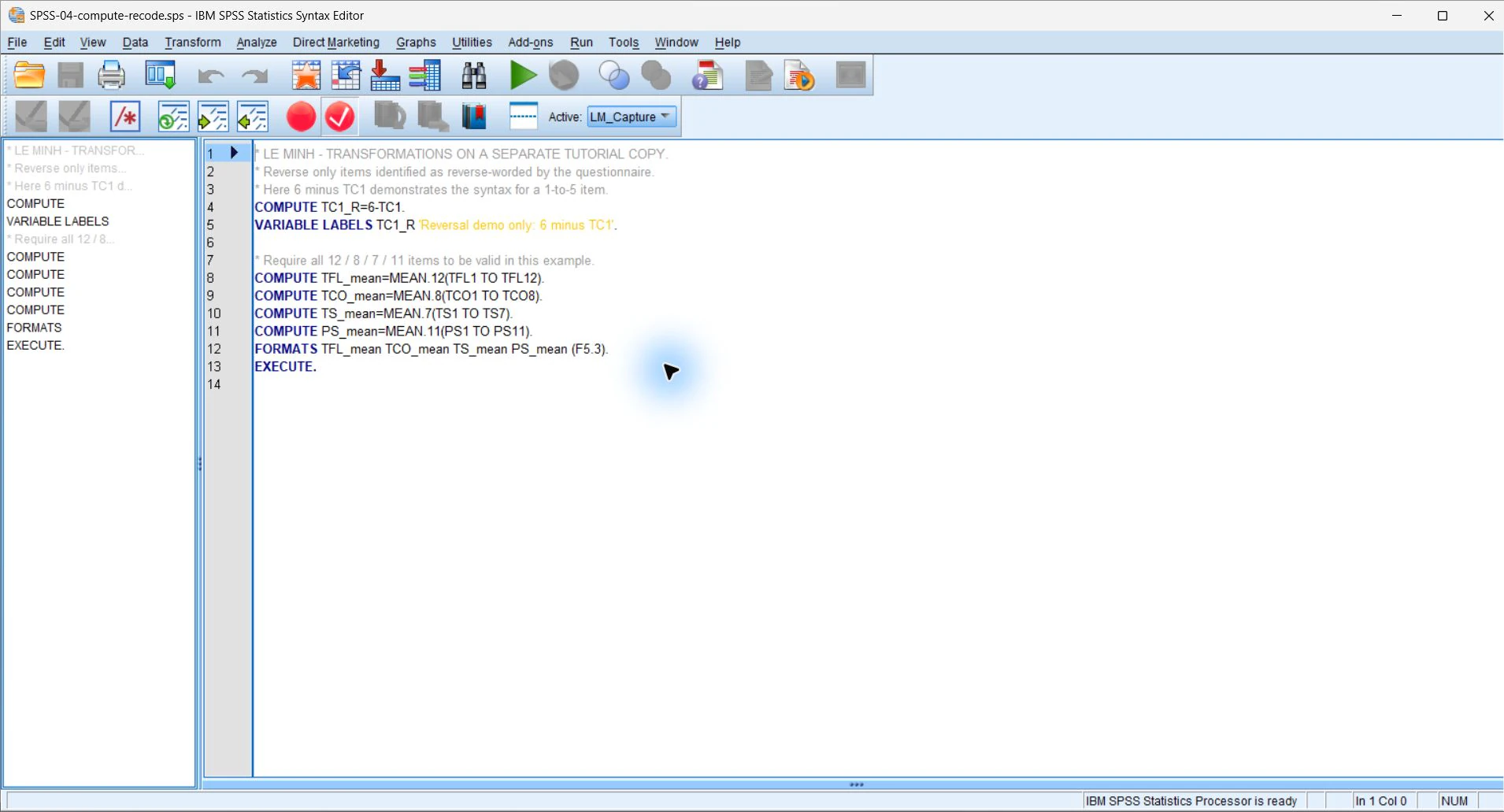
7. Check descriptives and reliability before the main model
Examine distributions, out-of-range values and indicator relationships before modeling. Cronbach's alpha does not replace assessing scale structure; it forms only part of reliability evidence.
Indicator removal requires substantive, measurement-quality and diagnostic reasons. Do not remove indicators solely for a slight alpha increase.
EXAMINE VARIABLES=satisfaction_mean trust_mean outcome
  /PLOT=HISTOGRAM NPPLOT
  /STATISTICS=DESCRIPTIVES
  /MISSING=LISTWISE.

RELIABILITY
  /VARIABLES=satisfaction1 satisfaction2_r satisfaction3 satisfaction4
  /SCALE('Satisfaction') ALL
  /MODEL=ALPHA
/STATISTICS=DESCRIPTIVE SCALE CORR.8. Estimate the model while preserving the research question
The regression below illustrates data flow only. Model, standard error and control-variable choices require research-design justification. Report coefficients, confidence intervals and conditions of application, rather than only p-values.
Command and subcommand order follow specific syntax rules. Consult Command Syntax Reference when commands fail or defaults need checking (IBM, n.d.-a).
| Output | Question to answer | Limitation to record |
|---|---|---|
| Coefficients | What are the coefficient's direction and magnitude? | Depends on coding, scales and specification |
| 95% CI | Which values are compatible with the data? | Not the probability that the parameter falls inside the interval |
| Residual plots | Are there signs of functional-form errors or heteroskedasticity? | Combine graphical diagnostics with theory |
| R squared | How much sample variation does the model explain? | Not equivalent to out-of-sample prediction |
REGRESSION
  /STATISTICS=COEFF OUTS R ANOVA CI(95)
  /DEPENDENT=outcome
  /METHOD=ENTER satisfaction_mean trust_mean age
  /RESIDUALS=HISTOGRAM(ZRESID) NORMPROB(ZRESID)
  /SAVE=PRED RESID.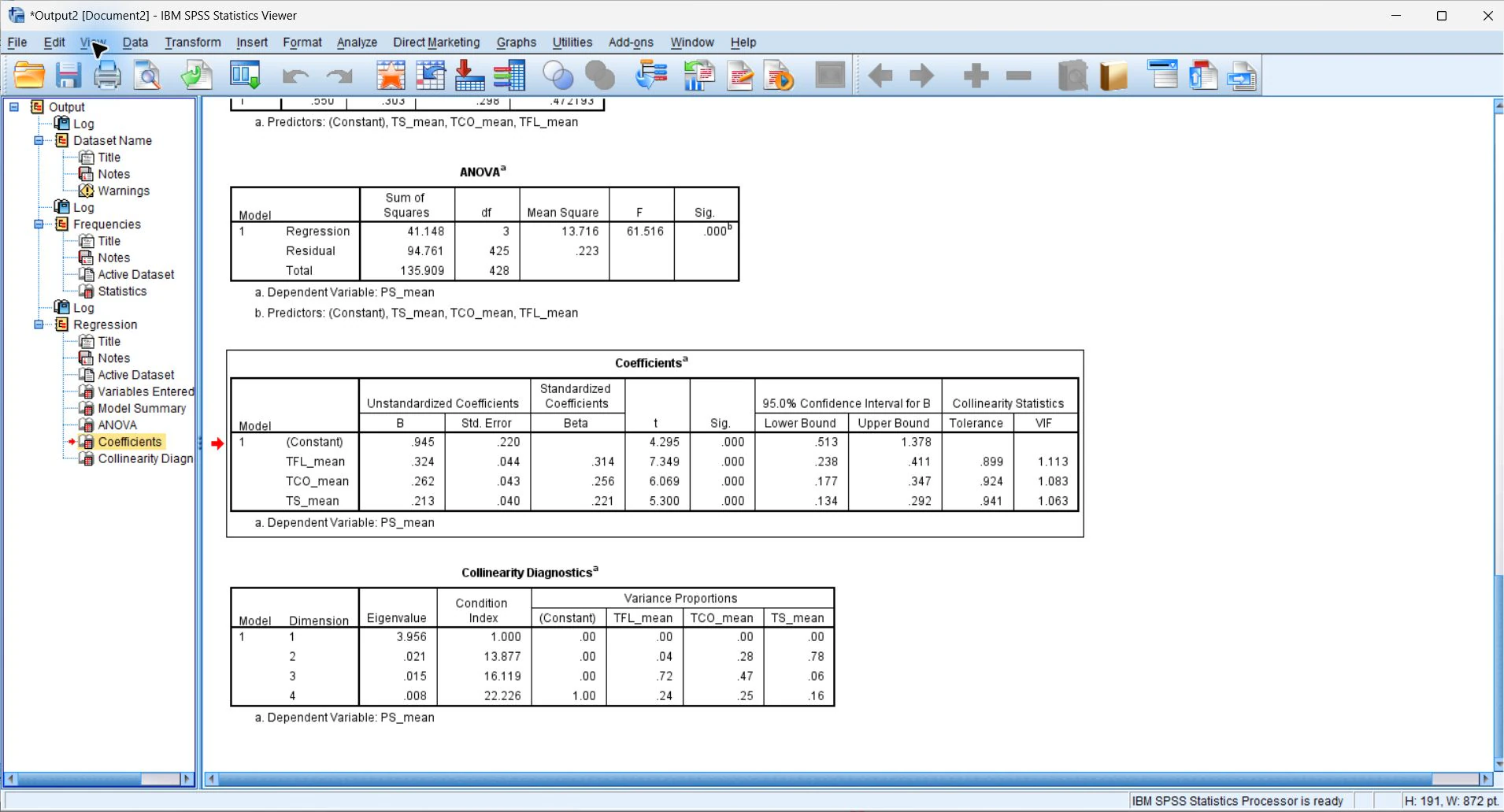
9. Rerun from the start and retain the audit trail
Close the dataset, open a fresh SPSS session and run syntax from the first line. If output cannot be recreated, the workflow is incomplete. Retain original output and a PDF for a durable format.
Pasting dialog selections into Syntax Editor is useful for learning commands. Read the syntax before running because dialog defaults may differ from the analysis plan.
Close the session
Ensure no dependence on temporary variables or undocumented actions.
Run all syntax
Monitor warnings, case counts and sample-size changes.
Check output
Confirm manuscript tables match the final run.
Save versions
Date or version syntax, derived data and output.
10. Reporting template and handover checklist
Example reporting paragraph
Data were processed in IBM SPSS Statistics [version]. Raw data were preserved unchanged; missing codes [description] were declared before variable creation. Scores for [scale] required at least [number] valid indicators under the registered rule. Model [name] was estimated on [N] cases. The coefficient for [X] was b = [ ], SE = [ ], 95% CI [ , ], p = [ ]. Diagnostic checks indicated [brief description and limitations].
- Raw data have not been overwritten.
- Codebook matches the questionnaire and Variable View.
- Missing codes are declared before scoring.
- Duplicate IDs, ranges and skip logic are checked.
- All recodes and computations have syntax.
- Case counts are recorded for every analysis.
- Reported tables trace to corresponding output and syntax.
- SPSS version and modules are specified.
Conclusion
A good SPSS workflow lets others move from raw data to the exact results table using the same commands. The interface speeds operations; syntax, codebook and decision logs make them auditable.
References
- IBM. (n.d.-a). Introduction to the Command Syntax Reference.https://www.ibm.com/docs/en/spss-statistics/32.0.0?topic=reference-introduction-guide-command-syntax
- IBM. (n.d.-b). Missing values: Overview (MISSING VALUES command).https://www.ibm.com/docs/en/spss-statistics/32.0.0?topic=values-overview-missing-command
- IBM. (n.d.-c). Missing Value Analysis.https://www.ibm.com/docs/en/spss-statistics/31.0.0?topic=values-missing-value-analysis
- Wilson, G., Bryan, J., Cranston, K., Kitzes, J., Nederbragt, L., & Teal, T. K. (2017). Good enough practices in scientific computing. PLOS Computational Biology, 13(6), e1005510.https://doi.org/10.1371/journal.pcbi.1005510
Academic note: MVA and some procedures depend on version or license. Consult documentation matching the IBM SPSS Statistics version in use. Example data and results illustrate the workflow only.