
Data Analysis Using R: A Workflow That Runs from Start to Finish
Code is useful only when it runs in a clean session, reads the correct inputs and recreates the reported tables or figures.
A reliable R workflow separates raw data, derived data, code and output; uses relative paths within an RStudio Project; checks assumptions through code; and records R and package versions. These practices reduce dependence on the analyst's hidden machine state (Posit Software, PBC, n.d.-a; Wilson et al., 2017).
A reproducible analysis workflow
- Codebook
Variable names, coding and missingness
- Preparation
Record data-cleaning steps
- Analysis
Keep configuration and analysis code
- Records
Save results and software versions
Conceptual diagram. Preserve original data and a change trail for verification.
Source: Lê Minh · Conceptual illustration, not software output.1. From isolated scripts to an analysis project
A script that runs on its author's computer may fail elsewhere because of absolute paths, leftover Environment objects, unrecorded package versions or data edited outside code.
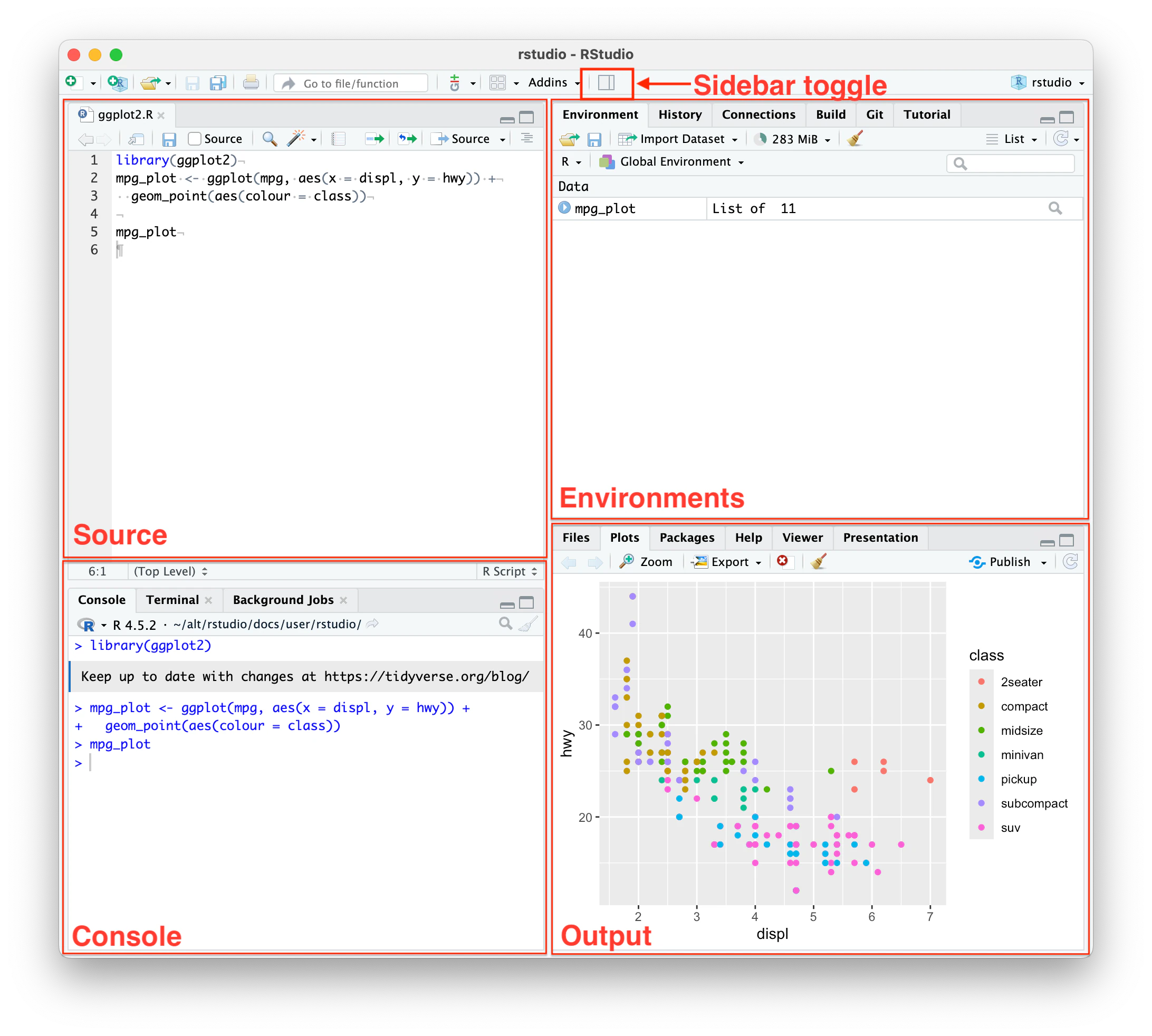
RStudio Projects provide stable root folders for code, data and outputs. Posit documentation recommends projects to separate working contexts and manage related files (Posit Software, PBC, n.d.-a).
Start a clean R session, open the project and run the main script. Recreating results without manual intervention passes the basic workflow check.
2. Folder structure and immutable data
Keep raw data in data/raw without overwriting it. Scripts create analysis data in data/derived and automatically generate tables and figures in output. This clearly separates inputs, transformations and products.
Do not store passwords, API keys or personally identifying data in code repositories. Keep sensitive data outside public repositories and explain access arrangements in README.
| Folder or file | Contents |
|---|---|
| data/raw/ | Original received data, read-only |
| data/derived/ | Script-generated data |
| R/ | Reusable functions |
| scripts/ | 01_import.R, 02_clean.R, 03_analysis.R |
| output/tables and output/figures | Automatically generated tables and figures |
| README.md | Execution order, inputs and outputs |
| renv.lock or environment description | Required package versions |
3. Start with a clean session
RStudio can restore earlier workspaces. Although convenient during exploration, hidden objects may let scripts succeed despite missing data-creation steps. Disable automatic .RData restoration and make scripts create every required object.
RStudio documentation describes workspace and startup settings. Agree these settings within the team and document them in README (Posit Software, PBC, n.d.-b).
# Run after opening the correct RStudio Project
getwd()

required_dirs <- c(
  "data/raw",
  "data/derived",
  "output/tables",
  "output/figures"
)

for (path in required_dirs) {
  if (!dir.exists(path)) dir.create(path, recursive = TRUE)
}

set.seed(20261025)Paths such as C:/Users/TenNguoiDung work on only one computer. Project-relative paths make code portable.
4. Import and check the data schema
Immediately check rows, names, types, unique IDs, ranges and missing counts after import. Do not wait for a model error before returning to these checks.
The example uses base R functions so readers can run it without installing packages. Code 99 becomes NA at import because the codebook defines it as user-missing.
raw <- read.csv(
  "data/raw/survey.csv",
  na.strings = c("", "NA", "99"),
  stringsAsFactors = FALSE
)

stopifnot("id" %in% names(raw))
stopifnot(!anyDuplicated(raw$id))

str(raw)
summary(raw)
colSums(is.na(raw))

likert_items <- c(
  paste0("satisfaction", 1:4),
  paste0("trust", 1:4)
)

range_errors <- vapply(
  raw[likert_items],
  function(x) sum(!is.na(x) & !(x %in% 1:5)),
  integer(1)
)

range_errors5. Declare data types and category labels
Numeric columns are not necessarily continuous. Gender codes 1, 2 and 3 are category labels. Converting them to factors prevents R from treating code differences as quantitative distances.
Factor ordering affects model reference groups. Specify levels and labels through code rather than relying on their order of appearance in a file.
analysis <- raw

analysis$gender <- factor(
  analysis$gender,
  levels = c(1, 2, 3),
  labels = c("Woman", "Man", "Self-described")
)

analysis$satisfaction2_r <-
  ifelse(
    is.na(analysis$satisfaction2),
    NA,
    6 - analysis$satisfaction2
)6. Calculate scale scores with transparent missingness rules
Using rowMeans with na.rm = TRUE can create a score from only one remaining indicator. This is often inappropriate for scales intended to cover several contents. The example requires at least three of four valid indicators.
The three-of-four rule is illustrative. Prespecify scoring from scale design, missingness and the analysis plan before examining results.
score_if_enough <- function(data, variables, min_valid) {
  values <- data[variables]
  n_valid <- rowSums(!is.na(values))
  score <- rowMeans(values, na.rm = TRUE)
  score[n_valid < min_valid] <- NA_real_
  score
}

analysis$satisfaction_mean <- score_if_enough(
  analysis,
  c("satisfaction1", "satisfaction2_r",
    "satisfaction3", "satisfaction4"),
  min_valid = 3
)

analysis$trust_mean <- score_if_enough(
  analysis,
  paste0("trust", 1:4),
  min_valid = 3
)7. Describe data and generate diagnostic plots
Descriptive tables should show valid counts, means, standard deviations, minima and maxima. Distribution plots reveal unusual values or structures that one summary cannot represent.
Do not use plots as automatic tests. Interpret them alongside measurement design and modeling objectives.
describe_one <- function(x) {
  c(
    n = sum(!is.na(x)),
    mean = mean(x, na.rm = TRUE),
    sd = sd(x, na.rm = TRUE),
    min = min(x, na.rm = TRUE),
    max = max(x, na.rm = TRUE)
  )
}

descriptives <- sapply(
  analysis[c("satisfaction_mean", "trust_mean", "outcome")],
  describe_one
)

write.csv(
  descriptives,
  "output/tables/descriptives.csv"
)

png("output/figures/outcome_histogram.png",
    width = 1600, height = 900, res = 150)
hist(analysis$outcome,
     main = "Distribution of outcome",
     xlab = "Outcome")
dev.off()8. Estimate models, confidence intervals and diagnostics
The illustrative regression below has a continuous outcome. This is not a default choice for all data. Formulas, control variables and missing-data handling must match the research question.
summary provides estimates and standard errors under model assumptions. confint adds confidence intervals. Diagnostic plots help inspect functional form, residuals and influential observations, but conclusions require several evidence sources.
fit <- lm(
  outcome ~ satisfaction_mean + trust_mean + age,
  data = analysis
)

summary(fit)
confint(fit, level = 0.95)

png("output/figures/model_diagnostics.png",
    width = 1600, height = 1600, res = 150)
par(mfrow = c(2, 2))
plot(fit)
dev.off()

model_table <- cbind(
  estimate = coef(fit),
  confint(fit, level = 0.95)
)

write.csv(
  model_table,
  "output/tables/model_coefficients.csv"
)9. Record the environment and rerun everything
R and package versions form part of the method. sessionInfo records operating system, R version and loaded packages; official manuals document base R function behavior (R Core Team, n.d.). For projects with many packages, lockfiles describe dependency versions.
Reproducibility also requires a clean-session check. Wilson et al. (2017) recommend automating repeated steps and documenting analysis dependencies.
write.csv(
  analysis,
  "data/derived/survey_analysis.csv",
  row.names = FALSE,
  na = ""
)

capture.output(
  sessionInfo(),
  file = "output/session-info.txt"
)

# Final check:
# 1. Restart R
# 2. Open the project
# 3. Run scripts in the order specified in README
# 4. Compare regenerated tables and figures10. Reporting template and handover checklist
Example reporting paragraph
Analyses used R [version] and packages [names and versions]. Raw data were preserved unchanged; analysis data were generated by scripts [names]. Missing codes [description] were converted to NA before scoring. Model [name] was estimated on [N] cases. The coefficient for [X] was b = [ ], SE = [ ], 95% CI [ , ], p = [ ]. Code, session information and outputs were retained with the analysis version.
- Scripts run from a clean R session.
- No absolute paths point to personal computers.
- Raw data are not overwritten.
- Types, ranges, IDs and missingness are checked through code.
- Scoring rules are explicit.
- Tables and figures are generated from analysis objects.
- Seeds are set for random steps.
- sessionInfo and package versions are retained.
- Sensitive data and credentials remain outside code repositories.
Conclusion
R is most valuable when every result comes from readable, rerunnable commands. A tidy project, unchanged raw data and automatically generated outputs help identify errors earlier and make handover clearer.
References
- Posit Software, PBC. (n.d.-a). RStudio projects.https://docs.posit.co/ide/user/ide/guide/code/projects.html
- Posit Software, PBC. (n.d.-b). RStudio IDE user guide.https://docs.posit.co/ide/user/index.html
- R Core Team. (n.d.). R manuals.https://cran.r-project.org/manuals.html
- Wilson, G., Bryan, J., Cranston, K., Kitzes, J., Nederbragt, L., & Teal, T. K. (2017). Good enough practices in scientific computing. PLOS Computational Biology, 13(6), e1005510.https://doi.org/10.1371/journal.pcbi.1005510
Academic note: The example uses base R to minimize dependencies. In real projects, record additional package versions and consult the manuals for functions in use. Example data and results are simulated.