
Descriptive Statistics in JASP: Checking Data, Selecting Measures, and Reporting Results
A table of means and standard deviations is not a complete descriptive analysis. Analysts must confirm variable types, missing data, distribution shapes and unusual cases before selecting the numbers to report.
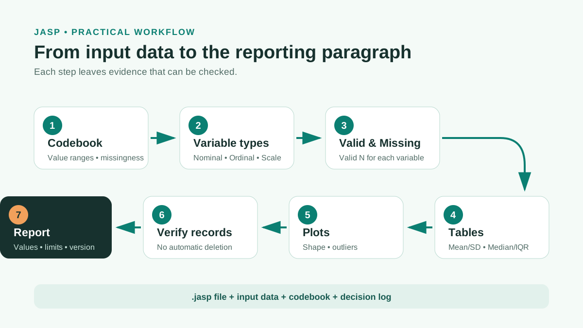
The practical workflow starts with a codebook and frozen dataset, continues with nominal, ordinal or scale declarations in JASP, and checks numerical summaries against plots. Record every processing decision and save the .jasp file with the software version.
1. Analysis objectives and required inputs
Descriptive statistics answer three questions: who is in the analysis sample, how each variable is distributed, and what data problems need resolving before inference. This is a data-checking stage, not merely a procedure for generating an introductory table.
Before opening JASP, prepare the raw data, codebook and missing-value coding rules. Each row should represent one observation unit defined by the design; every column needs a unique name, clear label and expected value range. Preserve an unchanged raw copy so later changes can be checked against it.
JASP updates results when options change and stores data with analyses in .jasp files. This helps review choices but does not replace a data-cleaning log or codebook (Love et al., 2019).
- The codebook matches the questionnaire or data source.
- The observation unit and identifier variable are known.
- Valid values and missing codes are defined.
- An unchanged raw dataset is retained.
- Variables to describe overall and by group are identified.
2. Declare nominal, ordinal and scale correctly
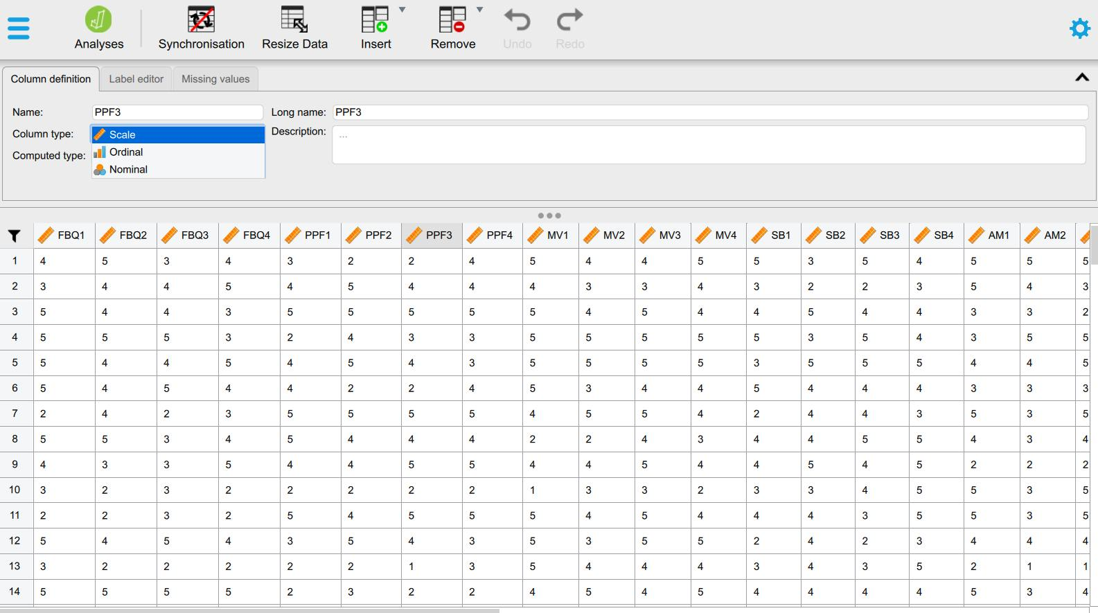
JASP needs the measurement role of every column. Nominal variables represent unordered groups; ordinal variables have ordered categories without guaranteed equal spacing; scale variables are analyzed as continuous. Codes 1, 2 and 3 do not turn a categorical variable into a continuous one.
An individual Likert item is inherently ordinal. A sum or average of multiple items is sometimes treated as scale, but that decision requires consideration of scale design, category count, distribution and analysis model. Do not change a variable's type merely to unlock a software option.
In JASP 0.98, the variable-type icon appears beside the column name. Interfaces may change across versions, so record the software version and check release notes when screenshots differ from your screen (JASP Team, 2026).
| Example | JASP type | Main summaries | Mistake to avoid |
|---|---|---|---|
| Gender, region | Nominal | n and % | Calculating means of group codes |
| Ordered education levels | Ordinal | n, %, median and quantiles where appropriate | Assuming equal spacing |
| Age in years | Scale | Mean, SD or median, IQR | Ignoring out-of-range values |
| Likert item from 1 to 5 | Ordinal | Category frequencies, median or justified summaries | Habitually calling the item continuous |
| Average of multiple items | Scale, with justification | Mean, SD, median, IQR and plots | Forgetting scoring rules for missing items |
3. Import and verify data before analysis
Open a CSV, Excel, SPSS or other supported file, then check row and column counts and several initial records against the source. For CSV files, verify delimiters, decimal marks and encoding. A numeric column read as text often signals unexpected characters, inconsistent decimal commas or untreated missing codes.
Avoid undocumented bulk edits in the data table. If editing in JASP, record the variable, old value, new value, reason and date. For larger projects, clean using syntax or tools with operation histories, then import the derived dataset.
The .jasp file should not be the only data copy. Save input data, codebook and analysis files separately. Goss-Sampson (2022) presents a workflow retaining data, choices and output in one JASP analysis session, but users must still manage file versions outside the software.
Open a data copy
Do not analyze the only raw file directly.
Verify dimensions
Record expected rows, columns and unique IDs.
Check column types
Confirm nominal, ordinal or scale against the codebook.
Check missing codes
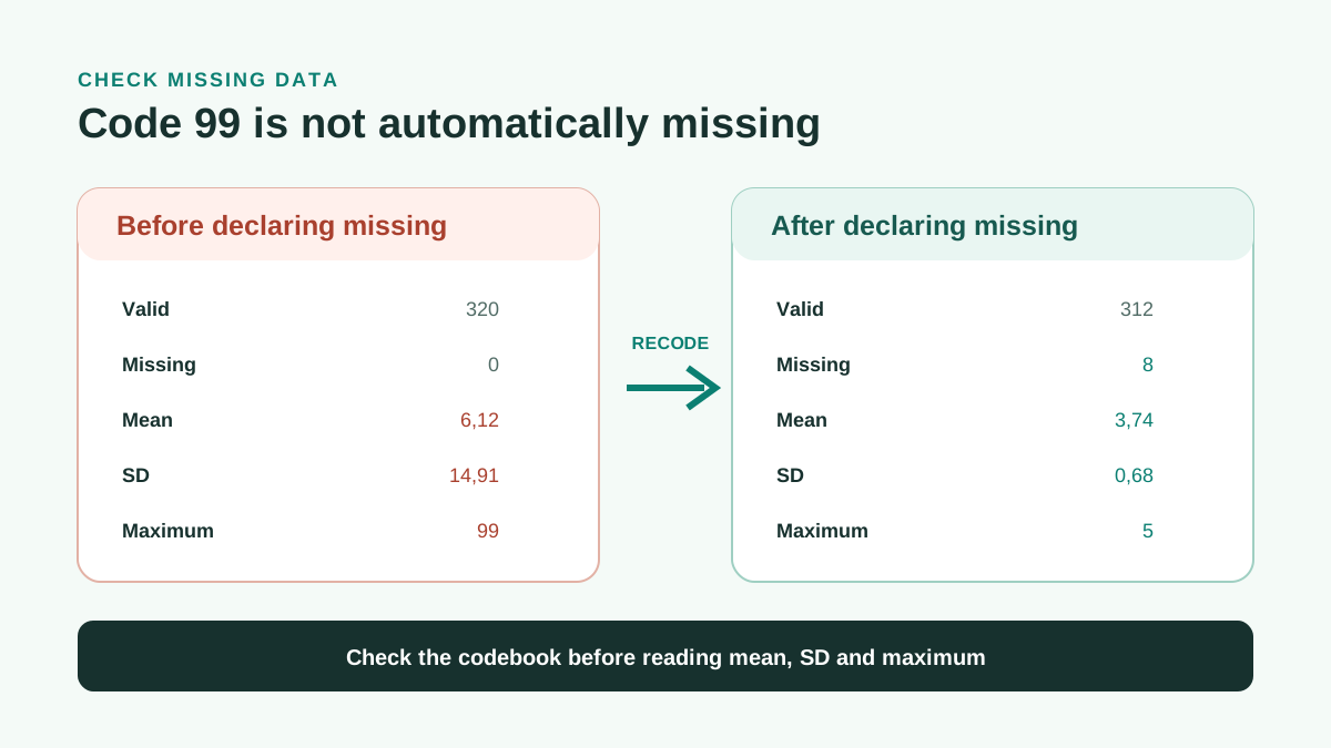
Ensure 99, 999 or NA strings are not treated as real values.
Save the analysis file
Use dated or versioned names, such as survey_descriptives_v01.jasp.
4. Use Descriptives in a controlled sequence
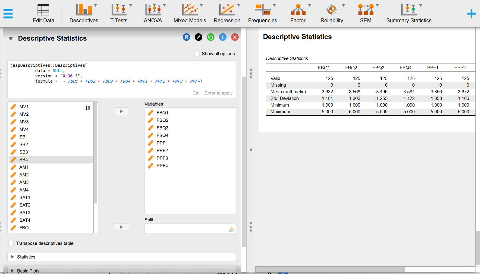
Open Descriptives, move target variables into Variables and add a group variable to Split when needed. Select Valid, Missing, Mean, Median, Standard deviation, IQR, Minimum, Maximum and relevant quantiles. Selecting every option is unnecessary: an overcrowded table can obscure the main problem.
Run the full sample before splitting by group. Descriptive values can fluctuate substantially in tiny groups and plots may mislead. Report valid observations for every variable because missingness changes sample sizes across columns.
Official Features and learning materials show that JASP supports descriptive statistics, distribution plots and many chart types. Option names can change between versions (JASP, n.d.-a; Goss-Sampson, 2022).
The demonstration places eight variables, FBQ1 to FBQ4 and PPF1 to PPF4, in one table for consistency checks. Displayed columns have 125 valid observations and no missing data; means range from 3,496 to 3,856 and standard deviations from 1,053 to 1,303. After this verification, select medians, IQRs, quartiles and distribution plots for the descriptive objective. These values illustrate reading output; they are not reference thresholds for other studies.
Select variables
Place similar variables together in Variables for readable tables.
Select counts
Always request Valid and Missing before measures of central tendency.
Select center and spread
Pair means with SDs and medians with IQRs or quantiles.
Select limits
Use minimum and maximum to detect out-of-range codes.
Add plots
Use histograms, density plots, boxplots, violins or Q-Q plots as appropriate.
Split groups when needed
Place the grouping variable in Split and check each group's N.
5. Choose summaries by variable type and distribution shape
Means and SDs are suitable for variables treated as scale when a few extreme values do not dominate the distribution. Medians and IQRs describe location and spread more robustly under skewness. Counts and percentages are the main outputs for nominal variables.
No single skewness or kurtosis threshold applies to all sample sizes and models. Read numerical summaries alongside histograms, boxplots, Q-Q plots and requirements of subsequent analyses. NIST/SEMATECH (2012) places plots at the center of exploratory data analysis because they reveal location, spread, skewness, outliers and multiple modes that one number cannot fully represent.
Shapiro-Wilk tests the normality hypothesis, but its p-value depends on sample size. Large samples can detect minor departures, while small samples may lack power. Do not use one p-value alone to delete data or change estimators (Ghasemi & Zahediasl, 2012).
| Situation | Main report | Supplement | Avoid |
|---|---|---|---|
| Nominal | n and % | Missing | Means of group codes |
| Few-category ordinal | n, %, median | IQR or quantiles | Reporting only means without category distributions |
| Approximately symmetric scale | Mean and SD | Min, max, CI or histogram | Concluding normality from similar mean and median alone |
| Skewed scale | Median and IQR | Quantiles, histogram, violin | Deleting tails to improve the mean |
| Scale with outliers | Both robust and conventional summaries | Boxplots and record checks | Deleting cases automatically labeled outliers |
6. Describe missing data before deciding how to handle it
Report missing counts and percentages for every variable. The total number of records is not always the N used for means or correlations. When missingness differs by variable, descriptive tables must show the corresponding valid Ns.
An undeclared code 99 distorts the mean, SD and maximum. Check maxima, frequency tables and codebook before interpreting distributions. After recoding missing values, rerun all Descriptives and save a new file.
Descriptive statistics do not establish whether missingness is MCAR, MAR or MNAR. Missing patterns by group, time or outcome require separate investigation. Do not replace missing values with means merely because JASP offers computed columns.
A Likert midpoint is a valid response when defined that way in the questionnaire. Nonresponse is missing data. These states require different codes.
7. Use boxplots to identify cases for checking, not automatic deletion
Boxplots commonly flag points outside fences based on 1,5 times the IQR. This is a screening rule, not proof of an erroneous observation. A value can be valid in a skewed distribution or belong to a real subgroup (NIST/SEMATECH, 2012).
Trace IDs to source records. Classify cases as entry errors, wrong units, sample-ineligible observations, valid rare observations or unresolved cases. Correct or exclude only under justified rules; retain a log explaining changes in N.
If valid outliers strongly affect results, report sensitivity analysis under appropriate specifications. Do not quietly exclude cases and present only favorable models.
| ID | Variable | Value | Verification source | Classification | Decision |
|---|---|---|---|---|---|
| A104 | Age | 222 | Original form says 22 | Entry error | Correct using a documented rule |
| B087 | Income | 350 | Correctly recorded in million VND/year | Valid but high | Retain and assess sensitivity |
| C015 | Scale from 1 to 5 | 9 | Original form unavailable | Out of range, unresolved | Set missing and report limitation |
8. Hypothetical example: satisfaction and usage time
These hypothetical data illustrate interpretation, not actual research findings. The file contains 320 respondents. Satisfaction is the average of four Likert items; usage time is measured in minutes.
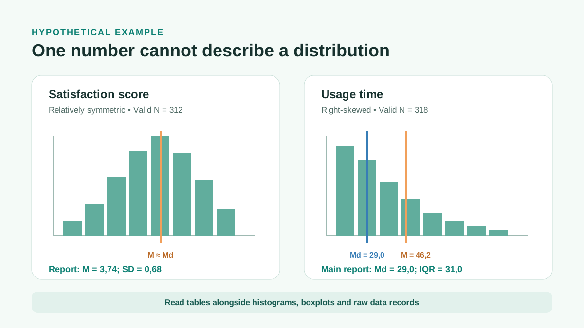
Satisfaction has valid N = 312, mean = 3,74, SD = 0,68, median = 3,75 and IQR = 1,00. The histogram is relatively symmetric without unusual gaps. Mean and SD can be reported alongside the eight missing cases.
Usage time has valid N = 318, mean = 46,2 minutes, SD = 51,8, median = 29,0 and IQR = 31,0. The histogram is right-skewed and the boxplot flags six high cases. Verification shows five valid cases and one value of 1.440 minutes caused by a unit error. Median and IQR are the main summaries before correction; corrected data must be described again.
A difference between mean and median does not prove a data error. It signals a need to examine plots and records. Wilkinson and the Task Force on Statistical Inference (1999) recommend checking data, plots and assumptions rather than relying on mechanical procedures.
| Variable | Valid N | Missing | Mean | SD | Median | IQR |
|---|---|---|---|---|---|---|
| Satisfaction | 312 | 8 | 3,74 | 0,68 | 3,75 | 1,00 |
| Usage time | 318 | 2 | 46,2 | 51,8 | 29,0 | 31,0 |
9. Describe groups without turning the table into a test
Split displays tables and plots by gender, intervention group, region or time. First check group Ns. Small groups can produce unstable SDs and sparse boxplots.
Descriptive sample mean differences are not evidence of population differences. If the question requires inference, use an appropriate model and report effect sizes and confidence intervals. Descriptives support understanding before model selection; they do not replace modeling.
Measurement equivalence may matter when comparing the same scale across groups. A lower mean does not necessarily imply a lower construct level if items function differently across groups.
Group tables describe observed sample data. Population conclusions require suitable sampling designs and inferential models.
10. Export tables, save files and retain reproducibility records
Save the .jasp file after finalizing data and options. Use versioned names and record JASP version and analysis date in a README or log. JASP Team (2026) recommends software citations containing the development team, year, version and software type.
Tables or plots can be copied to Word, but manuscript tables must trace to the correct .jasp file. When data change, reopen the file, refresh analyses and replace all affected output rather than manually editing numbers.
Instructional screenshots should conceal identifying data, remain legible and state the software version. Images do not replace copyable numerical tables or alternative content for screen-reader users.

- Data and .jasp filenames include versions.
- The JASP version appears in methods or README.
- Manuscript tables and figures trace to analysis files.
- Screenshots contain no personal data.
- Corrections, exclusions and recodes have a decision log.
11. APA 7 reporting template and pre-inference checklist
The template uses hypothetical practice values. Replace them with actual variables, Ns, missing counts, indices and selection rationales.
Example reporting paragraph
Data were checked in JASP 0.98 (JASP Team, 2026). Satisfaction had 312 valid observations and eight missing values, with M = 3,74 and SD = 0,68. The histogram indicated a relatively symmetric distribution. Usage time was right-skewed and was described by Md = 29,0 minutes and IQR = 31,0 minutes. Six boxplot-flagged cases were checked against raw records; five valid cases were retained and one unit error was corrected according to the data log. These values illustrate reporting only.
- Variable types match the codebook.
- Valid N and missingness are reported for each variable.
- Means are paired with SDs; medians with IQRs or quantiles.
- Numerical tables are read alongside plots.
- Outliers are traced to records rather than deleted automatically.
- Small-N groups are identified.
- .jasp files, input data and logs are retained with versions.
- Software is cited with its correct version.
Conclusion
Descriptive analysis in JASP should create an auditable data record: correct types, clear valid Ns, identified missing values, summaries suited to distributions and documented decisions for unusual cases.
Only then proceed to tests, regression, factor analysis or SEM. With incorrect input types or codes, a complex model merely makes errors harder to see.
References
- Ghasemi, A., & Zahediasl, S. (2012). Normality tests for statistical analysis: A guide for non-statisticians. International Journal of Endocrinology and Metabolism, 10(2), 486-489.https://doi.org/10.5812/ijem.3505
- Goss-Sampson, M. A. (2025). Statistical analysis in JASP: A guide for students (7th ed., Version 0.19.3).https://jasp-stats.org/wp-content/uploads/2025/07/Statistical-Analysis-in-JASP-A-guide-for-students-2025.pdf
- JASP. (n.d.-a). Features.https://jasp-stats.org/features/
- JASP Team. (2026). JASP (Version 0.98) [Computer software].https://jasp-stats.org/
- Love, J., Selker, R., Marsman, M., Jamil, T., Dropmann, D., Verhagen, J., Ly, A., Gronau, Q. F., Smíra, M., Epskamp, S., Matzke, D., Wild, A., Knight, P., Rouder, J. N., Morey, R. D., & Wagenmakers, E.-J. (2019). JASP: Graphical statistical software for common statistical designs. Journal of Statistical Software, 88(2), 1-17.https://doi.org/10.18637/jss.v088.i02
- NIST/SEMATECH. (2012). e-Handbook of statistical methods: Exploratory data analysis.https://www.itl.nist.gov/div898/handbook/eda/eda.htm
- Wilkinson, L., & Task Force on Statistical Inference. (1999). Statistical methods in psychology journals: Guidelines and explanations. American Psychologist, 54(8), 594-604.https://doi.org/10.1037/0003-066X.54.8.594
Academic note: Example values are hypothetical. Interface and option names were checked against JASP 0.98; users of other versions should consult release notes.