
SEM and GSEM in Stata: Choosing Commands, Specifying Models, and Interpreting Results
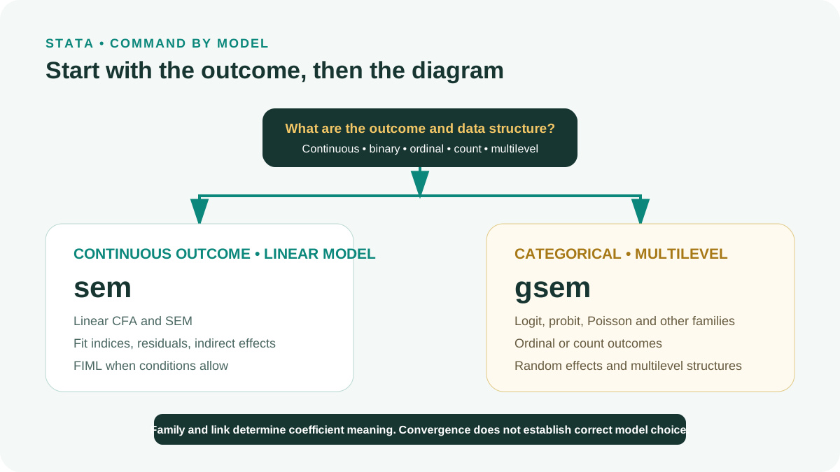
sem and gsem are not simply different levels of sophistication. Choose according to outcome type, measurement level, data structure, and the quantity the study seeks to interpret.
Use sem for linear systems and latent-variable models with continuous outcomes when assumptions are suitable; use gsem when outcomes require other families or links, or the model has generalized or multilevel structures. Each decision requires corresponding coefficient interpretation, missing-data handling, and diagnostics (StataCorp, 2025).
1. Start with the Dependent Variable Rather Than the Diagram
A diagram with many arrows does not justify gsem. Tabulate each equation: is the dependent variable continuous, binary, ordinal, or a count; are observations clustered; which variables are latent; and on which scale should coefficients be interpreted?
sem suits linear structural equation models within a covariance framework. gsem extends to other families and links and supports many generalized and multilevel structures. These extensions change coefficient meaning and available postestimation measures (Skrondal and Rabe-Hesketh, 2004; StataCorp, 2025).
| Situation | Starting command | Quantity to interpret |
|---|---|---|
| Continuous outcome, linear relationships | sem | Changes in original units or standardized coefficients |
| Binary outcome | gsem with logit or probit | Log-odds, odds ratios, or predicted probabilities |
| Ordinal outcome | gsem with ordered logit or probit | Thresholds and category probabilities |
| Count outcome | gsem with a suitable family | Log-counts or ratios of expected values |
| Generalized multilevel model | gsem | Fixed effects, random effects, and conditional predictions |
| Need linear SEM fit indices | sem if the model and data permit | Chi-square and supported fit indices |
Do not select logit, probit, Poisson, or negative binomial merely because estimation converges. Choices must match outcome support, the data-generating mechanism, and the research question.
2. Creating Do-Files, Logs, and Project Structure
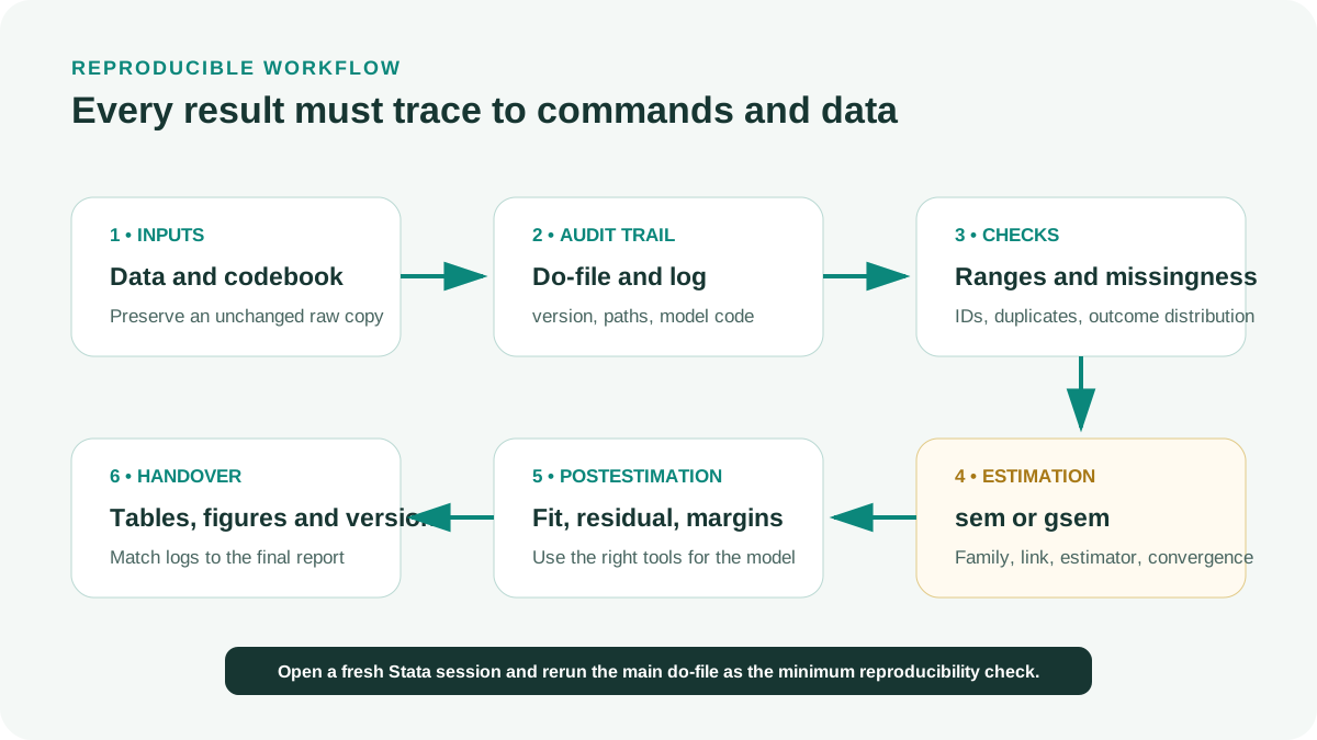
A do-file records all commands in order. A log saves commands and results as text. Stata documentation recommends do-files and logs to preserve an analysis trail (StataCorp, n.d.).
The version command makes Stata interpret syntax according to the specified release. Replace 19 with the version used for the final analysis. Relative paths make projects portable between computers.
| Path | Role |
|---|---|
| data/raw/ | Original data, unedited |
| data/derived/ | Data generated by do-files |
| do/ | 01_import.do, 02_clean.do, 03_model.do |
| output/ | Logs, tables, figures, and reports |
| docs/ | Codebook, README, and decision log |
version 19
clear all
set more off
capture log close _all

log using "output/analysis.log", text replace

import delimited "data/raw/survey.csv", ///
    varnames(1) encoding(utf8) clear

describe
codebook id gender age
isid id
duplicates report id3. Checking Data Before Model Specification
Model identification cannot repair basic coding errors. Before sem or gsem, check IDs, variable types, ranges, missing data, rare groups, and outcome distributions.
The following example treats 99 as missing according to its codebook. If 99 is valid in the actual data, replace would destroy information. Check the codebook first.
misstable summarize ///
    satisfaction1-satisfaction4 ///
    trust1-trust4 outcome

foreach v of varlist satisfaction1-satisfaction4 ///
                     trust1-trust4 outcome {
    replace `v' = . if `v' == 99
}

assert inrange(satisfaction1, 1, 5) ///
    if !missing(satisfaction1)

generate satisfaction2_r = 6 - satisfaction2 ///
    if !missing(satisfaction2)

egen satisfaction_mean = rowmean( ///
    satisfaction1 satisfaction2_r ///
    satisfaction3 satisfaction4)

egen n_satisfaction = rownonmiss( ///
    satisfaction1 satisfaction2_r ///
    satisfaction3 satisfaction4)

replace satisfaction_mean = . ///
    if n_satisfaction < 3

summarize satisfaction_mean outcome, detailEvery value-replacement command must follow the codebook or a verified data error. Do not change missing values or delete outliers merely to obtain convergence.
4. Model Specification and Identification
Establish identification before assessing fit. Each latent variable needs a scale, commonly by fixing a loading or variance. The path structure must provide enough information to estimate free parameters.
Identification is a property of the model and data rather than a technical option. Bollen (1989) presents SEM’s foundations of specification, identification, and estimation. If Stata reports nonidentification or an abnormal solution, check equations and measurement scales before adding constraints.
| Component | Question to address |
|---|---|
| Latent variables | Which indicators measure which constructs? |
| Scale | Which loading or variance is fixed? |
| Structural paths | Which paths have theoretical justification? |
| Correlated errors | Is there a substantive and design-based rationale? |
| Outcome | Which family and link are appropriate? |
| Missing | What information does the estimator use, and how are cases excluded? |
5. Practicing sem with Continuous Outcomes
The first example is an observed-variable path model. satisfaction_mean predicts trust_mean and outcome; trust_mean also predicts outcome. method(mlmv) illustrates maximum likelihood estimation with missing values supported by sem. Its applicability conditions must still be assessed.
estat gof provides fit indices after sem. Do not decide model correctness using one cutoff. Examine specification, residual magnitudes, parameter estimates, and theoretical plausibility.
sem ///
    (trust_mean <- satisfaction_mean age) ///
    (outcome <- trust_mean satisfaction_mean age), ///
    method(mlmv)

estat gof, stats(all)
estat stdize, all
estat teffects

estimates store sem_pathestat teffects suits linear sem models. In nonlinear gsem, multiplying two link-scale coefficients does not automatically yield a probability-scale indirect effect.
6. Practicing Measurement Models with sem
Stata latent variable names usually begin with uppercase letters to distinguish them from observed variables. The following example specifies two reflective constructs. By default, the first indicator of each construct sets its scale.
After estimation, check loadings, error variances, construct correlations, and residuals. A good fit index does not guarantee that indicators measure the intended conceptual content.
sem ///
    (Satisfaction -> ///
        satisfaction1 satisfaction2_r ///
        satisfaction3 satisfaction4) ///
    (Trust -> trust1 trust2 trust3 trust4), ///
    method(mlmv) standardized

estat gof, stats(all)
estat residuals, standardized

estimates store cfa_two_factor7. Practicing gsem with Ordinal Outcomes
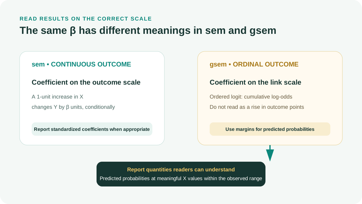
Suppose loyalty_level contains ordered categories. Ordered logit models cumulative probabilities through the logit link. The satisfaction_mean coefficient lies on the log-odds scale and should not be interpreted as a direct increase in loyalty points.
After gsem, many familiar sem fit indices cannot be used in the same way. Focus on family and link specification, convergence, estimates, prediction, and justified model comparisons (StataCorp, 2025).
gsem ///
    (loyalty_level <- ///
        satisfaction_mean trust_mean age), ///
    ologit vce(robust)

estimates store gsem_ordinal

margins, at( ///
    satisfaction_mean = (1 2 3 4 5) ///
) predict(outcome(4))

marginsplot, ///
    ytitle("Predicted probability") ///
    xtitle("Satisfaction mean")

graph export ///
    "output/figures/ordinal_probability.png", ///
width(1600) replacePredicted probabilities at meaningful values are often easier to interpret than raw logit coefficients. Values in at() must lie within the data range and suit the measurement scale.
8. Do Not Mechanically Compare sem and gsem Using One Number
Compare two models directly only when they describe the same outcome and sample and have a nesting relationship appropriate to the test. sem with a continuous outcome and gsem with an ordinal outcome specify different probability models.
If conclusions are sensitive to outcome treatment, present a sensitivity analysis. Explain why one specification is primary, what the other assesses, and which conclusions change.
| Aspect | sem | gsem |
|---|---|---|
| Coefficient scale | Outcome units or standardized | Link scale, odds ratios, or probabilities |
| Global fit | Linear SEM fit indices available | Do not apply the entire sem index set unchanged |
| Missing | Depends on the estimator and options | Depends on the family, estimator, and structure |
| Indirect effect | Linear effects can be used | Specify the scale and target quantity |
| Prediction | Fitted values on a continuous scale | Probabilities or expected values according to family |
9. Exporting Output and Verifying the Final Run
A complete do-file closes the log and saves derived data when needed. datasignature creates an identifier for the current data, helping detect file changes between runs.
Thesis tables must be traceable to saved models. When copying manually, record the estimates store name or model ID below the table for cross-checking.
Open a fresh Stata session
Do not rely on data or macros remaining in memory.
Run the main do-file
Record return codes, warnings, and case counts.
Cross-check the log
Verify that commands, estimator, and sample match the reporting tables.
Freeze the version
Save do-files, derived data, and output under one version identifier.
compress
save "data/derived/survey_analysis.dta", replace

datasignature set, reset
datasignature report

estimates dir
log close10. Reporting Template and Checklist
Example report
The model was estimated in Stata [version] using [sem/gsem]. For equation [name], the outcome was modeled using family [ ] and link [ ]; standard errors were calculated using [ ]. The analysis sample comprised [N] cases after applying the missing-data rule [description]. The coefficient for [X] was b = [ ], SE = [ ], 95% CI [ , ], p = [ ]. On the interpretation scale [units/log-odds/probability], this corresponds to [interpretation]. Identification, convergence, and sensitivity checks indicated [brief description].
- Classify each outcome by support and measurement scale.
- Provide a methodological rationale for sem or gsem.
- State the family, link, estimator, and standard-error method.
- Check latent-variable scaling and identification conditions.
- Report missing data and case counts for each model.
- Interpret coefficients on the correct scale.
- Do not apply sem fit cutoffs to gsem.
- Ensure the do-file runs from a fresh session and save the log.
- Clearly label example data or hypothetical results.
Conclusion
Choosing sem or gsem precedes software operation. Once outcomes, families, links, and interpretation targets are clear, syntax becomes a verifiable description of the model. Do-files, logs, and derived data make results traceable.
References
- Bollen, K. A. (1989). Structural equations with latent variables. Wiley.https://doi.org/10.1002/9781118619179
- Skrondal, A., & Rabe-Hesketh, S. (2004). Generalized latent variable modeling: Multilevel, longitudinal, and structural equation models. Chapman & Hall/CRC.https://www.routledge.com/Generalized-Latent-Variable-Modeling-Multilevel-Longitudinal-and-Structural/Skrondal-Rabe-Hesketh/p/book/9780429205491
- StataCorp. (n.d.). Stata User's Guide.https://www.stata.com/manuals/u.pdf
- StataCorp. (2025). Stata 19 Structural Equation Modeling Reference Manual. Stata Press.https://www.stata.com/manuals/sem.pdf
Academic note: Syntax and postestimation can change by release. Replace version 19 with the actual version and consult its Stata manual. The example data, variable names, and results are simulated.