
Interpreting R², Adjusted R², f², Q², and PLSpredict Correctly in PLS-SEM
R², f², and Q² are not three different names for effect magnitude. They answer three different questions about explanation, unique contribution, and prediction.
Interpret R² and f² in the structural model, then use PLSpredict to assess out-of-sample prediction. Blindfolding Q² has historical value but does not replace Q²predict, RMSE, MAE, or the CVPAT test.
Explanation and prediction answer different questions
- R² / adjusted R²
Explained variance in the sample
- f²
The predictor’s unique contribution
- PLSpredict
Errors on held-out observations
- CVPAT
Compare predictive losses
Conceptual diagram. High R² alone does not establish out-of-sample prediction.
Source: Lê Minh · Conceptual illustration, not software output.1. What Should You Be Able to Do After This Article?
This guide is designed to help readers open a SmartPLS 4 report and independently answer four questions: how much variance the model explains in each endogenous variable, how much each predictor contributes, whether the model predicts better than a simple benchmark, and how to report the results in a thesis or article. Cite the software used in the workflow according to the developer’s information (Ringle et al., 2024).
You need a PLS-SEM model whose measurement model assessment is complete. If reliability, convergent validity, or discriminant validity is inadequate, pause structural-model interpretation because R², f², and prediction indices rely on construct scores that have not yet been adequately supported.
- Clearly identify the endogenous variable to be explained or predicted.
- Complete the assessment of the reflective or formative measurement model.
- Run the PLS-SEM Algorithm and bootstrapping using the same model specification.
- Know whether the study’s primary objective is explanation, prediction, or both.
2. A Map of the Indices: Each Answers a Different Question
R² and adjusted R² describe the variance explained in the sample. f² measures the change in R² when a predictor is removed from the equation. Blindfolding Q² assesses predictive relevance through a data-point omission procedure, whereas Q²predict in PLSpredict compares out-of-sample prediction errors with a mean-based prediction benchmark (Hair and Alamer, 2022; Shmueli et al., 2019).
Do not place these indices in one table and simply conclude that the model is good. A model with a respectable R² can still predict poorly out of sample. Conversely, a variable with a statistically significant path coefficient can have a very small f² if its unique contribution to explained variance is negligible.
| Index | Question addressed | Unit of interpretation | Must not be interpreted as |
|---|---|---|---|
| R² | How much variance in Y do the exogenous variables explain? | Each endogenous variable | Evidence of out-of-sample prediction |
| Adjusted R² | How much R² remains after accounting for the number of predictors and sample size? | Each endogenous variable | A statistical significance test |
| f² | How much does Y’s R² decrease when X is removed from the equation? | Each path X → Y | The magnitude of the path coefficient |
| Q² blindfolding | Does the model have predictive relevance under the omission procedure? | Each endogenous variable | Prediction of new data |
| Q²predict | Does PLS-SEM predict better than the mean benchmark? | Each endogenous indicator | A direct comparison with the LM model |
| RMSE or MAE | Are PLS-SEM prediction errors lower than the benchmark? | Each indicator or latent variable | Causal meaning |
3. Formulas to Understand Before Opening the Software
R² is the proportion of an endogenous variable’s variance explained by the predictor set. Adjusted R² penalizes the addition of unnecessary variables and is therefore often more appropriate when comparing two models with different numbers of predictors.
The f² effect size is calculated as f² = (R² full - R² excluded)/(1 - R² full). It measures the loss of explained variance when a predictor is removed. Values of 0,02, 0,15, and 0,35 are commonly used to describe small, medium, and large effects, but should be treated as guidance rather than rigid boundaries (Cohen, 1988).
Q²predict is calculated from the ratio of the sum of squared PLS-SEM prediction errors to the sum of squared errors of the mean benchmark. Positive Q²predict indicates that PLS-SEM predictions have lower errors than this benchmark. It does not yet show that PLS-SEM outperforms the linear model LM; that requires a direct comparison of the two models’ RMSE or MAE (SmartPLS, n.d.-a).
| Index | General formula | Interpretation |
|---|---|---|
| R² | 1 - SSE/SST | Proportion of Y’s variance explained in the sample |
| Adjusted R² | 1 - (1 - R²)(n - 1)/(n - k - 1) | Adjusts for sample size n and number of predictors k |
| f² | (R² full - R² excluded)/(1 - R² full) | X’s unique contribution to Y’s R² |
| Q²predict | 1 - SSE PLS/SSE mean benchmark | A positive value means PLS outperforms the mean benchmark |
Formulas help check the logic and identify misread tables. For formal reporting, use the values calculated by SmartPLS from the correct model and configuration. Do not combine R² from one run with an excluded-variable R² from a different model.
4. A Hand-Calculated f² Example and Its Interpretation
The example below is illustrative and does not report an actual study. Suppose that Continued Use Intention has R² = 0,520 in the full model. Removing Trust reduces R² to 0,470. Removing Service Quality reduces R² to 0,505.
For Trust, f² = (0,520 - 0,470)/(1 - 0,520) = 0,104. For Service Quality, f² = (0,520 - 0,505)/(1 - 0,520) = 0,031. According to Cohen’s (1988) guidelines, both are small effects, but Trust makes a unique contribution approximately three times that of Service Quality.
Do not claim that Trust has three times the effect on the basis of these two f² values alone. f² compares changes in explained variance, not the ratio of two path coefficients.
| Variable removed | Full-model R² | Excluded-variable R² | f² | Interpretation |
|---|---|---|---|---|
| Trust | 0,520 | 0,470 | 0,104 | Small effect, with a more substantial unique contribution |
| Service Quality | 0,520 | 0,505 | 0,031 | Small effect |
| Price | 0,520 | 0,519 | 0,002 | Negligible contribution |
5. Interpreting R² and Adjusted R² in Context
R² ranges from 0 to 1 and never decreases when predictors are added. A higher R² therefore does not automatically establish that a model is better. If many predictors are added while adjusted R² remains almost unchanged, the extension may offer little additional explanatory value.
R² assessment thresholds depend on the field, the stability of the phenomenon, the research design, and the model’s objectives. A moderate R² may be reasonable in consumer behavior, where decisions are influenced by many factors outside the model. Report each endogenous variable’s value and interpret it contextually rather than labeling it good or poor solely from the software’s colors (SmartPLS, n.d.-b).
If R² = 0,52, the correct statement is that the predictor set explains 52% of the endogenous variable’s variance in the sample. Do not state that the model is 52% accurate, that 52% of respondents exhibit the behavior, or that this establishes causality.
6. Interpreting f² Alongside Path Coefficients and Confidence Intervals
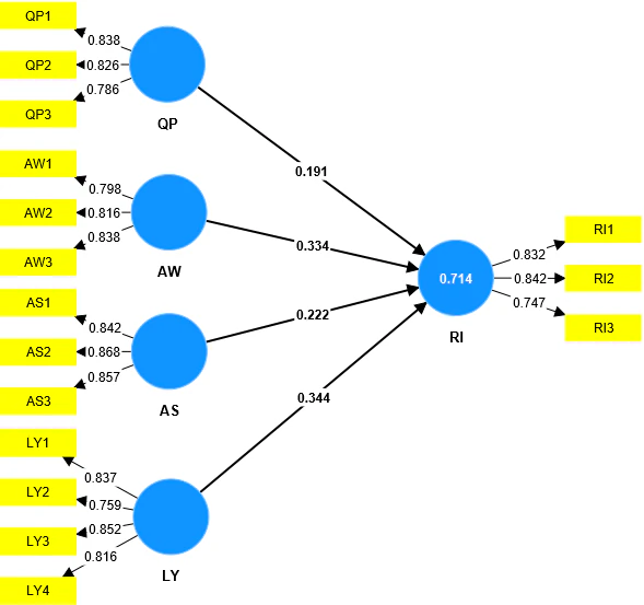
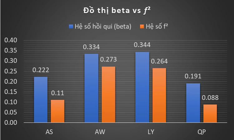
A standardized path coefficient indicates the direction and magnitude of a relationship conditional on the other variables in the equation. Bootstrapping indicates estimation uncertainty. f² answers another question: how much does Y’s explanatory R² decrease if X is removed?
A path with p < 0,05 but f² < 0,02 may be statistically significant while making a very small practical contribution. A nonsignificant path with a wide confidence interval should not be retained merely because f² exceeds 0,02. Interpret coefficients, confidence intervals, f², and theory together.
| Bootstrap result | f² | Cautious interpretation |
|---|---|---|
| Significant | 0,02 or higher | Evidence of a relationship and a unique contribution under the reference guideline |
| Significant | Below 0,02 | A relationship may exist, but its explanatory contribution is very small |
| Nonsignificant | 0,02 or higher | Examine confidence intervals, power, multicollinearity, and model specification |
| Nonsignificant | Below 0,02 | No substantial empirical evidence in this sample |
7. Distinguishing Blindfolding Q², Q²predict, and CVPAT
Blindfolding Q² is obtained by systematically omitting some data points and re-estimating the model. It was previously used to assess in-sample predictive relevance, but it is not an out-of-sample prediction test based on training and held-out data.
PLSpredict divides the data into folds, estimates the model using the training portion, and predicts the held-out portion. Positive Q²predict indicates that PLS-SEM outperforms the mean benchmark. Next, compare PLS-SEM’s RMSE or MAE with the LM model for each endogenous indicator. SmartPLS now also provides CVPAT to test differences in predictive ability rather than merely compare errors descriptively (SmartPLS, n.d.-a; Shmueli et al., 2019).
RMSE penalizes large errors more strongly and is appropriate when the prediction-error distribution is relatively symmetric. MAE is less sensitive to extreme errors. Do not select a measure after viewing the results to obtain a favorable conclusion; specify the criterion in advance and report consistently.
| Result | Meaning | Next step |
|---|---|---|
| Q²predict > 0 | PLS-SEM outperforms the mean benchmark | Compare RMSE or MAE with LM |
| Q²predict ≤ 0 | The mean benchmark performs as well as or better than PLS-SEM | Do not conclude that this indicator has predictive ability |
| PLS RMSE/MAE < LM | The theoretical model predicts this indicator better than the LM benchmark | Synthesize results across all endogenous indicators |
| PLS RMSE/MAE ≥ LM | LM predicts equally well or better | Review specification and avoid claims of strong prediction |
| CVPAT p < 0,05 and lower PLS loss | The test provides evidence of a difference in predictive ability | Report the benchmark type and loss |
8. A Practical Workflow in SmartPLS 4
Menu names may change slightly between SmartPLS 4 updates, but the logic of interpretation remains the same. Retain one model specification throughout the workflow so the tables can be compared.
Run the PLS-SEM Algorithm
Open Calculate and select PLS-SEM Algorithm. After running it, go to Quality criteria and record R-square and R-square adjusted for each endogenous variable.
Open the f-square table
Under Quality criteria, select f-square and switch to Matrix if needed. Read the correct cell where the predictor’s row intersects the endogenous variable’s column.
Run bootstrapping
Read the path coefficients, confidence intervals, and p-values. Check coefficient signs and whether confidence intervals include 0 before considering f².
Run PLSpredict
Open Calculate and select PLSpredict. Check the number of folds, repetitions, and random seed. The default of 10 folds is a starting point, but each fold must leave enough observations for stable estimation.
Interpret results against two benchmarks
Read Q²predict for the comparison with the mean benchmark. Then select RMSE or MAE and compare PLS-SEM with LM for each endogenous indicator.
Check CVPAT if available
Identify the benchmark, loss type, and direction of the difference before reading the p-value. p < 0,05 is useful only when PLS-SEM’s loss is lower than the benchmark’s.
Colors in SmartPLS reports help identify results against preset thresholds. Theses and articles must present the values, criteria, sources of the criteria, and interpretations within the study’s context.
9. A Self-Assessment Exercise
Suppose a model predicts Loyalty from Satisfaction, Trust, and Switching Costs. The illustrative Loyalty results are R² = 0,610 and adjusted R² = 0,602. Removing Trust reduces R² to 0,550. For indicator LOY1, Q²predict = 0,180, PLS-SEM RMSE = 0,720, and LM RMSE = 0,760.
These values give Trust an f² of (0,610 - 0,550)/(1 - 0,610) = 0,154. This can be described as a medium effect using Cohen’s reference guidelines. Positive Q²predict and lower PLS-SEM RMSE than LM for LOY1 provide favorable predictive evidence for this indicator. Do not conclude that the entire model has high predictive ability until the remaining endogenous indicators have been checked.
- Recalculate f² and compare it with 0,154.
- Explain the 0,008 difference between R² and adjusted R².
- Check Q²predict before comparing PLS-SEM with LM.
- Do not generalize the LOY1 result to the entire scale without examining the other indicators.
- Write a results paragraph that clearly separates in-sample explanation from out-of-sample prediction.
10. APA 7 Reporting Template and Final Checklist
The template below uses the exercise’s hypothetical values. For an actual study, replace all bracketed values with the original results and use a consistent number of decimal places.
Example report
The model explained 61,0% of the variance in Loyalty (R² = .610; adjusted R² = .602). Trust had a positive effect on Loyalty, β = [coefficient], 95% bootstrap confidence interval [lower bound, upper bound], p = [value], with an effect size of f² = .154. PLSpredict results for LOY1 indicated Q²predict = .180; PLS-SEM RMSE (.720) was lower than the LM model’s (.760). This result supports out-of-sample predictive ability for LOY1. Conclusions about the overall Loyalty construct were drawn after comparing all endogenous indicators.
- Report R² and adjusted R² for each endogenous variable.
- Associate f² with the correct path and do not equate f² with β.
- Report bootstrap confidence intervals, not only p-values.
- State the number of folds, repetitions, random seed, and PLSpredict error measure.
- Compare each indicator against the mean benchmark and LM.
- Separate conclusions about in-sample explanation from conclusions about out-of-sample prediction.
- Check that every in-text citation has a corresponding reference-list entry.
Conclusion
The correct workflow has two layers. The explanatory layer uses R², adjusted R², path coefficients, and f². The predictive layer uses PLSpredict, Q²predict, RMSE or MAE, and CVPAT where appropriate.
No single index is sufficient to label a model good. A conclusion is credible only when indices are interpreted in relation to the correct question, unit, and limitations of the research design.
References
- Cohen, J. (1988). Statistical power analysis for the behavioral sciences (2nd ed.). Lawrence Erlbaum Associates.https://doi.org/10.4324/9780203771587
- Hair, J., & Alamer, A. (2022). Partial least squares structural equation modeling (PLS-SEM) in second language and education research: Guidelines using an applied example. Research Methods in Applied Linguistics, 1(3), 100027.https://doi.org/10.1016/j.rmal.2022.100027
- Ringle, C. M., Wende, S., & Becker, J.-M. (2024). SmartPLS 4 [Computer software]. SmartPLS.https://www.smartpls.com
- Shmueli, G., Sarstedt, M., Hair, J. F., Cheah, J.-H., Ting, H., Vaithilingam, S., & Ringle, C. M. (2019). Predictive model assessment in PLS-SEM: Guidelines for using PLSpredict. European Journal of Marketing, 53(11), 2322-2347.https://doi.org/10.1108/EJM-02-2019-0189
- SmartPLS. (n.d.-a). PLSpredict: Assessing predictive power in PLS-SEM.https://www.smartpls.com/documentation/algorithms-and-techniques/prediction-and-segmentation/predict/
- SmartPLS. (n.d.-b). Result color thresholds in SmartPLS reports.https://www.smartpls.com/documentation/functionalities/thresholds/
Academic note: The numerical examples in this article illustrate calculations and interpretation; they are not actual research data. Thresholds provide reference guidance and do not replace theory, research design, or assessment of uncertainty.