
PLS-MGA and MICOM in SmartPLS 4: Evidence-Based Group Comparisons
A path that is significant in group A but nonsignificant in group B does not establish a difference between the groups. Multigroup analysis must directly test the difference and is meaningful only when measurement invariance has been assessed.
The correct workflow begins with a group-difference hypothesis and group definitions, assesses sample size and each group’s model, conducts MICOM, and then uses permutation or PLS-MGA to test parameter differences. Conclusions must state each group’s coefficient, the difference, p-value, and procedure name.
Group comparisons start with equivalence
- Define groups
Explicit theory and group coding
- Measurement invariance
Check whether comparisons are valid
- Compare paths
Test the difference directly
- Interpretation
Report sample sizes and limitations
Conceptual diagram. Different p-values do not by themselves establish different coefficients.
Source: Lê Minh · Conceptual illustration, not software output.1. What Should You Be Able to Do After This Article?
Readers should be able to distinguish MGA from continuous moderation, create groups without distorting the data’s meaning, assess the three MICOM steps, run permutation and PLS-MGA in SmartPLS 4, and correctly interpret each procedure’s p-values. Report the software version and cite it in the methods section (Ringle et al., 2024).
Inputs include a predefined grouping variable, a hypothesis identifying which parameters are expected to differ, a common PLS-SEM model for all groups, a coding codebook, and sufficient observations in each group. Total sample size does not replace assessment of power and stability in the smallest group.
- Groups must have theoretical or design-based meaning and must not be created after examining results.
- A hypothesis or question must identify the parameters to be compared.
- Each observation must belong to exactly one group, with no missing group codes.
- Use the same model, indicators, coding, and algorithm settings across groups.
- Check sample size and data quality separately for each group.
- Decide between PLS-SEM and PLSc-SEM before selecting the corresponding permutation procedure.
2. What Does MGA Test?
MGA directly tests whether the same parameter, such as a path coefficient, outer loading, or outer weight, differs across predefined groups. Sarstedt et al. (2011) show that MGA procedures differ in assumptions and construction of their test distributions, so reports must identify the method used.
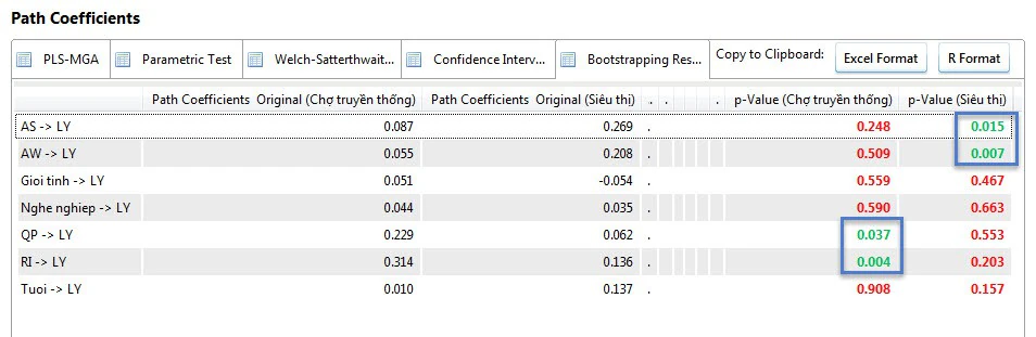
MGA cannot be performed by comparing two separate p-values. A coefficient with p = 0,03 in group A and p = 0,12 in group B may still show no significant between-group difference because the standard error and distribution of the difference have not been tested.
The test must directly target H0: beta_A - beta_B = 0. Conclude that a difference exists only when MGA or permutation rejects this hypothesis at the prespecified alpha level.
3. Defining Groups and Checking Data Before Analysis
Natural or design-based groups, such as countries, intervention groups, or customer types, suit MGA when clearly defined and coded. Splitting continuous variables at the mean or median loses information, reduces power, and makes results dependent on the cutoff. If the hypothesis concerns a continuous variable changing a slope, an interaction term is usually more appropriate.
Before comparison, tabulate observation counts, missing data, the grouping-variable distribution, sample characteristics, and indicator quality for each group. Each group’s model must converge without serious problems; good full-sample results do not guarantee adequacy in a small group.
| Research question | Method to consider | Consideration |
|---|---|---|
| Does the same path differ between two predefined groups? | MGA after MICOM | Directly test the difference |
| Does a continuous variable change the slope? | Continuous moderation | Retain continuous-variable information |
| Are there unobserved segments? | FIMIX-PLS or PLS-POS | Exploratory segments require further validation |
| Are there more than two groups? | Planned comparisons or an omnibus approach | Control the number of tests and hypotheses |
4. Why MICOM precedes MGA
A path difference may reflect different score composition rather than a different structural mechanism. MICOM assesses PLS-SEM composites; it does not replace within-group measurement evaluation and is not a copy of multigroup CFA (Henseler et al., 2016).
Configural and compositional evidence supports partial invariance. A model-wide comparability claim requires examining all relevant composites. Step 3 additionally examines mean and variance equality; full invariance does not establish equal paths or automatically justify replacing group analyses with pooled results (Hair et al., 2018, Chapter 4).
| Step | Evidence | Not a substitute |
|---|---|---|
| 1. Configural | Shared indicators, treatment and estimation configuration | An output p-value |
| 2. Compositional | Observed c versus its permutation distribution | A high c alone or a rounded value of 1 |
| 3. Mean/variance | Observed differences inside reference intervals | Only checking whether zero lies inside |
5. Reading MICOM in SmartPLS 4
SmartPLS (n.d.-a) includes MICOM in the permutation report; Step 1 requires configuration records. At Step 2 and alpha = .05, compare c with the fifth percentile of its permutation distribution, retaining enough precision for the decision. A single-item c of 1 is not evidence of reliability (Hair et al., 2018, Chapter 4).
At Step 3, compare the observed mean difference and log variance ratio with their corresponding permutation intervals. An interval may contain zero while excluding the observed difference. Check this distinction when reconciling a book, output and older interpretations (Hair et al., 2018, Chapter 4; SmartPLS, n.d.-a).
Prepare a construct-level table before reading paths. If composition is unsupported for a construct, comparisons involving it lack the necessary invariance evidence. Increasing permutations cannot repair coding or specification errors; justify corrections and rerun the sequence (Hair et al., 2018, Chapter 4).
The MICOM guide develops step-by-step interpretation, including an interval that contains zero but excludes the observed difference. This guide continues from a defensible invariance scope to direct tests of between-group coefficient differences.
6. Workflow in SmartPLS 4
Permutation and PLS-MGA both use groups created within the dataset. For standard PLS-SEM, use standard permutation; for a PLSc-SEM model, use consistent permutation so comparisons rely on the same algorithm (SmartPLS, n.d.-b).
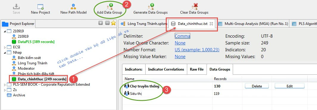
Create data groups
Open the dataset, create filters based on group codes, and verify the actual observation count in each group.
Run the model separately for each group
Assess the measurement model, structural model, convergence problems, and unusual indicators within each group.
Open Calculate > Permutation
Select Group A and Group B, the prespecified test type, alpha, and number of permutations.
Use 5.000 permutations for final results
SmartPLS defaults to 1.000; official documentation suggests larger numbers such as 5.000 for more stable final results.
Assess MICOM first
Record configural, compositional, partial, or full invariance conclusions for each composite.
Read permutation MGA
Report group coefficients, the observed difference, permutation p-value, and direction of the difference.
Run PLS-MGA when a cross-check is needed
Use bootstrap groups and interpret p according to the PLS-MGA rule rather than the permutation rule.
Save settings and output
Record the software version, algorithm, bootstrap count, permutation count, test type, alpha, and missing-data treatment.
7. Distinguish permutation and PLS-MGA
Permutation exchanges observations between groups, preserves group sizes and refits the model to form a reference distribution of differences. Specify a one- or two-sided test from the planned hypothesis, rather than changing direction after inspecting coefficient signs. Hair et al. (2018, Chapter 4) distinguish this procedure from the bootstrap-distribution comparisons used in PLS-MGA.
Under the SmartPLS PLS-MGA reporting convention, p < .05 or p > .95 is flagged at the 5% level (SmartPLS, n.d.-c). These tails concern the procedure's directional representation, not a rule for every p-value column. Do not call p = .98 an ordinary two-sided p-value. For a nondirectional difference hypothesis, prespecifying a two-sided permutation test gives a clearer interpretation (Hair et al., 2018, Chapter 4).
State the A − B ordering and verify the convention of the selected output column. The difference's magnitude and sign identify the comparison direction; p does not replace them. Parametric and Welch-Satterthwaite tests have different assumptions and should not be selected because one gives the smallest p (Sarstedt et al., 2011).
| Procedure | Reference distribution | Interpretation to report |
|---|---|---|
| Two-sided permutation | Differences after group-label permutation | Two-sided p against the prespecified alpha |
| PLS-MGA | Group-specific bootstrap estimates | Directional convention; verify tail and A/B ordering |
| Parametric / Welch-Satterthwaite | Statistics and SE under each test's assumptions | Name the test and assumptions; do not use the p > .95 convention |
8. Hypothetical Numerical Example: Trust and Continuance Intention
The example below is illustrative rather than client data. Suppose a study compares new and long-term users. MICOM establishes partial invariance for Trust and Continuance Intention, permitting comparison of standardized paths across the two groups.
The Trust-to-Continuance Intention coefficient is 0,42 for new users and 0,18 for long-term users. The A - B difference is 0,24. A two-sided permutation test with 5.000 permutations gives p = 0,022; PLS-MGA gives p = 0,018. Both illustrative procedures support a difference, with a stronger relationship among new users.
| Parameter | Group A | Group B | A - B | Permutation p | PLS-MGA p |
|---|---|---|---|---|---|
| Trust -> Continuance Intention | 0,42 | 0,18 | 0,24 | 0,022 | 0,018 |
| Quality -> Trust | 0,55 | 0,49 | 0,06 | 0,438 | 0,401 |
A p-value only addresses compatibility with the null hypothesis of no difference. Practical conclusions require considering the magnitude 0,24, confidence intervals, each group’s power, and the theoretical rationale for the direction of the difference.
9. More groups and paths increase the testing family
With g groups there are g(g − 1)/2 group pairs. Testing h paths across every pair produces h × g(g − 1)/2 tests. Four groups and three paths create 18 tests, rather than one isolated question at alpha = .05. Hair et al. (2018, Chapter 4) explain why searching many pairs increases false-positive risk.
Define the hypothesis family and necessary comparisons before analysis. Asking whether any group differs requires an appropriate overall test; a set of unadjusted pairwise tests is not automatically an omnibus test. Do not run an ordinary ANOVA on bootstrap coefficients as if each resample were an independent participant (Hair et al., 2018, Chapter 4).
The chapter discusses overall tests and pairwise adjustments. Verify which procedure the available software actually supports; an old book interface does not establish a current SmartPLS menu. For pairwise reporting, retain the full testing family, raw p-values and adjustment rule, including unfavorable results.
10. Constructed example: a conclusion changes after Holm adjustment
Suppose three planned path-difference hypotheses form one testing family and use two-sided permutation. Their illustrative p-values are .012, .026 and .210. These are constructed reporting inputs, not values derived from three pairs of betas. R's p.adjust implements Holm adjustment to control familywise error (R Core Team, n.d.).
The adjusted values are .036, .052 and .210. At alpha = .05, the second hypothesis no longer meets the criterion within this family. Do not pass only p-values already below .05 to the function, since that changes the family after inspecting results. This example uses two-sided p-values, not the raw directional PLS-MGA column.
| Planned comparison | Permutation p | Holm p | Read at alpha = .05 |
|---|---|---|---|
| Path 1, A − B | 0.012 | 0.036 | Still meets the criterion |
| Path 2, A − B | 0.026 | 0.052 | Does not meet it after adjustment |
| Path 3, A − B | 0.210 | 0.210 | Does not meet the criterion |
# Constructed two-sided permutation p-values for one planned family.
p <- c(path1 = 0.012, path2 = 0.026, path3 = 0.210)
result <- data.frame(raw_p = p, holm_p = p.adjust(p, method = "holm"))
print(result)
stopifnot(isTRUE(all.equal(unname(result$holm_p), c(0.036, 0.052, 0.210))))
choose(4, 2) * 3 # 18 pairwise path tests across four groups
0.42 - 0.18      # 0.24, difference in the earlier constructed example
11. Unequal group sizes and robustness
A large total sample does not remove a small group's uncertainty. Report usable observations, measurement quality, estimation diagnostics and uncertainty for each group. Hair et al. (2018, Chapter 4) note that substantial size imbalance can affect test performance; this calls for design and sensitivity assessment, not automatic deletion of large-group observations.
A nonsignificant result is not evidence of group equivalence. Inspect the difference and its uncertainty where available, and state what size of difference matters in the research context. If trying alternative specifications or sample rules, keep the question and testing family consistent and report both primary and sensitivity analyses.
Groups discovered by FIMIX/PLS-POS from the same data remain exploratory. A subsequent MGA on that dataset is not independent confirmation of stable market segments. Interpretation needs group content and evidence beyond the segmentation procedure (Hair et al., 2018, Chapter 5).
9. Common Errors in Group Comparisons
| Weak practice | Problem | Remedy |
|---|---|---|
| p_A < 0,05 and p_B > 0,05, so the groups differ | The difference has not been tested directly | Use permutation or PLS-MGA |
| Omitting MICOM | Differences may be measurement artifacts | Report the three invariance steps before MGA |
| Median-splitting a continuous variable | Loss of information and power | Use continuous moderation if it matches the hypothesis |
| Justifying adequacy using total sample size | The smaller group may lack power | Assess each group and the target parameter |
| Testing many paths and selecting small p-values | Increased risk of chance findings | Prespecify comparisons and adjust where necessary |
| Calling all p-values PLS-MGA | Conceals differences between procedures | Correctly identify permutation, PLS-MGA, or the parametric test |
13. APA-style reporting text and completion checklist
Connect the MICOM evidence to the difference test actually used. Identify comparable composites, the A/B ordering and the hypothesis family; if reporting several procedures, keep their interpretations separate (Hair et al., 2018, Chapter 4; Sarstedt et al., 2011).
Suggested reporting text
MICOM used [number] permutations in SmartPLS 4 (Ringle et al., 2024). Configuration was documented through [records]. Composition was supported for [list] but not for [list]; MGA was restricted to [scope]. The X → Y coefficient was beta = [ ] in Group A (n = [ ]) and beta = [ ] in Group B (n = [ ]), giving A − B = [ ]. The [named, one-/two-sided] test returned raw p = [ ]. Within the family of [number] planned hypotheses, [adjustment rule or reason for no adjustment] gave reported p = [ ]. Interpretation considered magnitude, uncertainty and group-size limitations. Any supplementary PLS-MGA result was identified separately under its directional convention.
- State the grouping rationale and reference coding.
- Report group sizes, missingness and model quality.
- Document Step 1 and retain Step 2 results for each composite.
- Distinguish partial/full evidence and unsupported comparisons.
- Record permutations, bootstrap runs, test type, alpha and seed where available.
- Report each group coefficient and the A − B direction.
- Separate directional PLS-MGA p from two-sided p.
- Retain the complete testing family, raw p and adjustment rule.
- Do not infer a difference from separate group p-values.
- Discuss magnitude, uncertainty, power and robustness.
Conclusion
PLS-MGA is useful when group differences are formulated as research questions before analysis. Groups must be meaningful, each group’s model must be adequate, and MICOM must indicate whether composites are formed equivalently.
Final conclusions depend on directly testing the difference, not on one group having a small p-value while the other has a large one. A good report shows each group’s coefficient, the difference, procedure name, p-value, invariance conditions, and sample-size limitations.
References
- Henseler, J., Ringle, C. M., & Sarstedt, M. (2016). Testing measurement invariance of composites using partial least squares. International Marketing Review, 33(3), 405-431. https://doi.org/10.1108/IMR-09-2014-0304
- Sarstedt, M., Henseler, J., & Ringle, C. M. (2011). Multigroup analysis in partial least squares (PLS) path modeling: Alternative methods and empirical results. In M. Sarstedt, M. Schwaiger, & C. R. Taylor (Eds.), Measurement and research methods in international marketing (Vol. 22, pp. 195-218). Emerald. https://doi.org/10.1108/S1474-7979(2011)0000022012
- Ringle, C. M., Wende, S., & Becker, J.-M. (2024). SmartPLS 4 [Computer software]. SmartPLS. https://www.smartpls.com
- SmartPLS. (n.d.-a). Measurement invariance assessment (MICOM). https://smartpls.com/documentation/algorithms-and-techniques/heterogeneity-and-multigroup/micom/
- SmartPLS. (n.d.-b). Permutation testing for PLS-SEM multigroup analysis. https://www.smartpls.com/documentation/algorithms-and-techniques/resampling-and-inference/permutation/
- Hair, J. F., Sarstedt, M., Ringle, C. M., & Gudergan, S. P. (2018). Advanced issues in partial least squares structural equation modeling. SAGE. https://us.sagepub.com/en-us/nam/advanced-issues-in-partial-least-squares-structural-equation-modeling/book243803
- SmartPLS. (n.d.-c). Multigroup analysis (MGA) in PLS-SEM with SmartPLS. https://smartpls.com/documentation/algorithms-and-techniques/heterogeneity-and-multigroup/multigroup-analysis/
- R Core Team. (n.d.). p.adjust: Adjust p-values for multiple comparisons. R documentation, stats package. https://stat.ethz.ch/R-manual/R-devel/library/stats/html/p.adjust.html
Methodological note: The example values illustrate output interpretation. Actual MGA conclusions depend on measurement invariance, group formation, sample size, power, estimation algorithm, and prespecified hypotheses.