
Modification Indices in AMOS: Diagnosing Misspecification Without Chasing Model Fit
A Modification Index is not a list of instructions for revising a model. It is a local diagnostic for a currently fixed parameter and is useful only when that parameter has theoretical meaning, practical magnitude, and potential for validation using other data.
A careful workflow checks the solution and residuals, reads MI alongside expected parameter change, identifies the type of misspecification, examines variable content, frees at most one parameter at a time, re-estimates the entire model, and documents every post hoc change.
1. Learning Objectives and Prerequisites for Examining MI
After this guide, you should explain what MI measures, retrieve the correct AMOS table, distinguish residual covariances, cross-loadings, and structural paths, read MI alongside Parameter Change, and decide whether to retain or revise a model using a verifiable decision log.
Inspect MI only after the model is identified, estimation has converged, and no improper solution is present. MI cannot repair root causes such as miscoded data, an excessively small sample, serious distributional violations, or an unclear initial theoretical model (Brown, 2015).
- Finalize a theoretically grounded model before estimation.
- Ensure there are no identification errors, negative variances, or impossible loadings.
- Examine overall fit and standardized residuals.
- Check each item’s content and coding direction.
- Save the original model before making changes.
- Plan to validate the modified model using another sample or sensitivity analysis.
2. What Does a Modification Index Actually Measure?
MI is a score-test statistic for a currently fixed parameter, usually fixed at 0. Under suitable approximation conditions, it predicts the reduction in chi-square if that parameter alone is freed and the model is re-estimated (Sörbom, 1989). A large MI indicates that a constraint may be inconsistent with the data, but does not establish the substantive correctness of the change.
Each MI is a local diagnostic conditional on the entire current model. After a parameter is freed, the remaining MIs may change substantially. Do not add multiple MIs to predict the fit improvement from several changes or simultaneously free every top-ranked parameter.
The threshold 3,84 is sometimes used because of its relationship to a one-df chi-square test at 0,05. It is not a parameter-selection rule. Both MI and chi-square difference tests are sample-size sensitive: with large n, minor misspecification can still produce a significant statistic. Interpret MI with EPC, residuals, and substantive meaning rather than p-values alone (Kline, 2023). MI tables usually contain many tests, so scanning dozens or hundreds of rows increases the risk of modifying the model to fit sample noise.
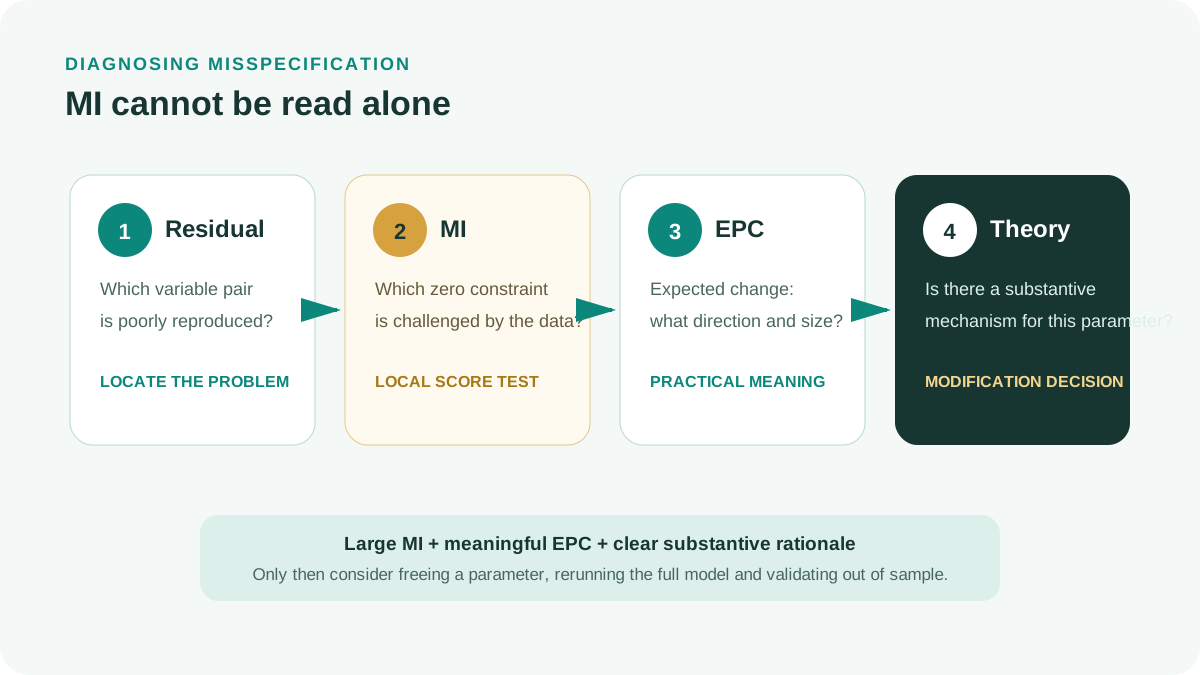
A large MI may reflect cross-loadings, similar item content, wording effects, omitted variables, mixed sample groups, or an incorrect constraint. Data alone cannot choose among these explanations in place of theory.
3. Interpreting MI Alongside Expected Parameter Change
MI primarily reflects statistical evidence against an existing constraint. Expected Parameter Change (EPC), usually labeled Par Change in AMOS, predicts the parameter’s magnitude and direction if freed. Rows with similar MIs can have very different EPCs and therefore different practical priorities.
Unstandardized EPC depends on measurement scales. Standardized Expected Parameter Change (SEPC) makes magnitudes easier to compare across parameter types. Whittaker (2012) shows that standardized EPC can provide more useful parameter-selection information than MI ranking alone.
If MI is large but EPC is tiny, a change may improve chi-square because of sample size without practical importance. If both MI and EPC are substantial but the parameter contradicts theory, retaining the model and discussing the discrepancy may still be appropriate.
| MI | EPC or SEPC | Substantive rationale | Preliminary decision |
|---|---|---|---|
| Small | Small | Present or absent | Do not prioritize modification |
| Large | Small | Weak | Possible sample-size effect; retain the model |
| Large | Substantial | Strong | Consider one change and re-estimate |
| Large | Substantial | Absent | Do not free merely to improve fit |
| Moderate | Substantial | Strong | Check residuals, wording, and stability |
4. Enabling and Reading Modification Indices in AMOS
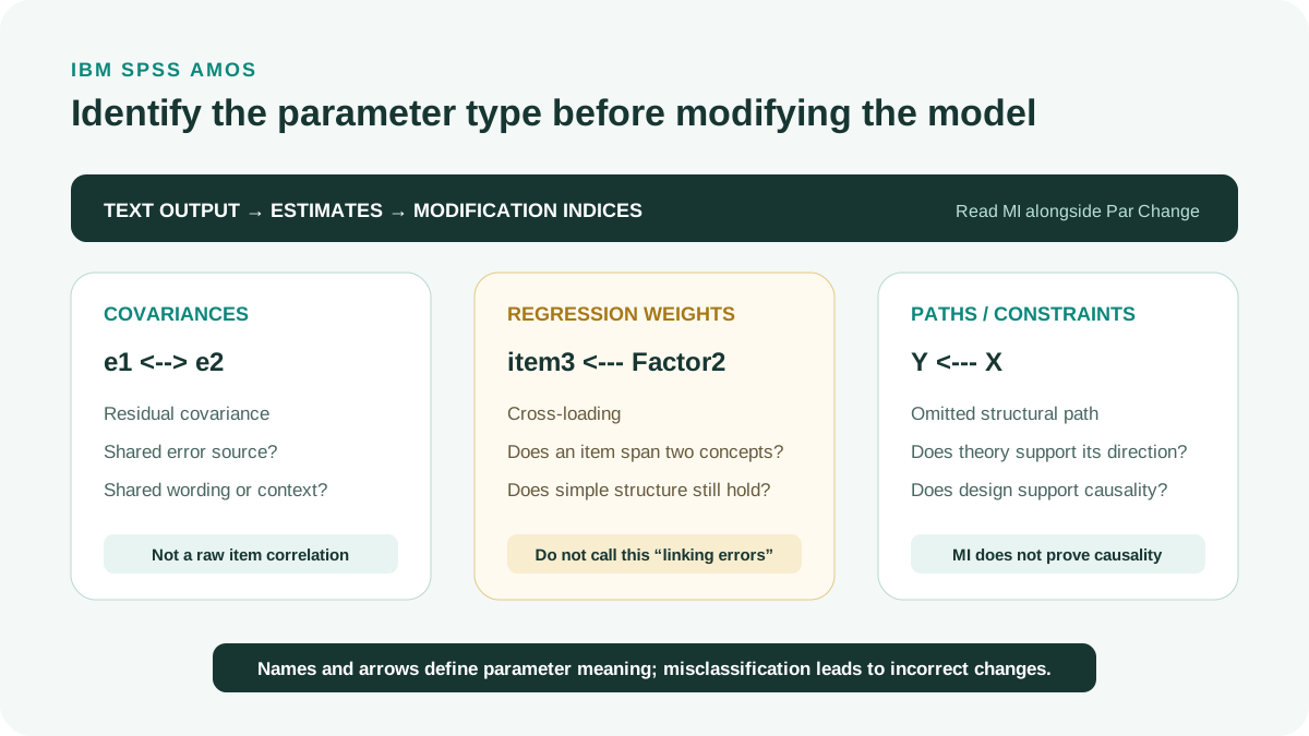
In IBM SPSS Amos 29 Graphics, open Analysis Properties, select Output, enable Modification indices, and enter a display threshold if needed. After estimation, open Text Output and locate Modification Indices. IBM Corp. (2022) describes enabling this table in the AMOS 29 guide.
AMOS divides the table into covariances, variances, and regression weights. In CFA, common suggestions include error correlations and an indicator’s cross-loading onto another factor. In structural models, it may suggest an omitted regression path.
Read variable names carefully. The row e1 <-> e2 represents a residual covariance rather than a correlation between two observed items. The row item3 <--- Factor2 represents a cross-loading. These modifications have different measurement meanings and should not both be described simply as adding arrows.
Save the original model
Create a dated, version-named copy before enabling MI.
Enable Modification indices
Under Analysis Properties > Output, select MI and retain Standardized estimates and Residual moments.
Estimate the unmodified model
Save the initial model’s fit indices, residuals, loadings, correlations, and warnings.
Classify each suggestion
Label each row as a residual covariance, cross-loading, structural path, or other constraint.
Read MI alongside Par Change
Record the magnitude, sign, and units of the expected change.
Cross-check variable content
Review wording, data collection, and theory before deciding.
5. From a Large MI to a Misspecification Hypothesis
A large residual-covariance MI may arise when items share wording, examples, reverse-coding formats, or an unmodeled method source. Correlated errors are reasonable only when a specific shared mechanism beyond the main factor exists.
A large cross-loading MI suggests that an item may also measure another factor. Before adding a cross-loading, examine wording and conceptual definitions. If an item is genuinely ambiguous, revising or removing it in a subsequent study may be clearer than retaining a difficult-to-interpret model.
A large structural-path MI may suggest an omitted variable, a direct relationship beyond mediation, or an inappropriate causal ordering. Cross-sectional data do not independently establish causal direction, so adding paths must begin with theory and research design.
Unusual variance or covariance MIs sometimes signal inappropriate equality constraints, particularly in multigroup models. Examine the invariance objective rather than randomly freeing parameters.
| MI row | Diagnostic hypothesis | Question to address | Risk of mechanical modification |
|---|---|---|---|
| e1 <-> e2 | Shared error source | Do the items share wording or context? | Conceals cross-loadings or method factors |
| item <--- another factor | Cross-loading | Does the item’s content belong to two concepts? | Loses CFA simple structure |
| Y <--- X | Omitted structural path | Do theory and measurement timing support this direction? | Rationalizes a post hoc relationship |
| Equality constraint | Noninvariance or parameter differences | Which constraint is being tested? | Undermines the meaning of group comparisons |
6. A Controlled Model-Modification Workflow
Data-driven specification searches can produce a model that fits the current sample but replicates poorly. MacCallum (1986) cautions that models generated through searching must be treated as post hoc. The objective is therefore to identify explainable, verifiable misspecification rather than obtain the most attractive indices.
Free only one theoretically approved parameter per iteration. Then re-estimate the entire model and check the solution, fit, residuals, loadings, correlations, and new MIs. If the change produces abnormal coefficients or weakens conceptual meaning, return to the previous model.
Verify the initial model
Check identification, convergence, Heywood cases, fit, and residuals before MI.
Select the discrepancy region
Use standardized residuals to locate variable pairs or model regions with poor covariance reproduction.
List relevant MIs
Retain only suggestions within the discrepancy region that have a plausible substantive interpretation.
Read EPC or Par Change
Discard changes with negligible magnitudes or implausible signs.
Write the rationale before modifying
Record a sentence explaining the parameter-generating mechanism and supporting literature or wording.
Free one parameter
Create a new model version without overwriting the original.
Re-estimate the entire model
Check every parameter, fit, and residuals rather than only the chi-square decrease.
Validate stability
Prefer a holdout sample, cross-validation, or an independent sample; if unavailable, explicitly state the exploratory nature.
If the next suggestion is justified only by a large MI or the desire to meet a cutoff, stop the workflow. Improved fit cannot compensate for a model that no longer has a coherent interpretation.
7. Hypothetical Numerical Example: Two Similarly Worded Items
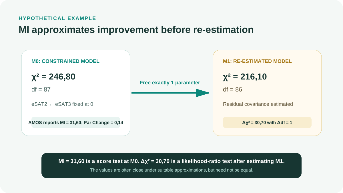
The following example is illustrative rather than actual research data. A three-factor CFA model has chi-square = 246,80 with df = 87. The standardized residual between SAT2 and SAT3 is 0,19. AMOS reports MI = 31,60 for eSAT2 <-> eSAT3 and Par Change = 0,14.
Both items begin with the same phrase, use the same service example, and are adjacent in the questionnaire. The team anticipated a wording effect in the design log, providing a substantive rationale for residual covariance. After freeing exactly one covariance, chi-square decreases to 216,10 with df = 86. Because M1 is nested in M0 and only one additional parameter is freed, Δχ² = 246,80 - 216,10 = 30,70 with Δdf = 1 is the likelihood-ratio chi-square difference test for the two nested models.
MI is a score test, whereas Δχ² is a likelihood-ratio test after re-estimation. Both have asymptotic one-df chi-square distributions in this example, but MI uses information only at the constrained solution to approximate improvement. Δχ² uses two fully estimated solutions. Thus, MI = 31,60 is close to but need not equal the actual decrease of 30,70 (Sörbom, 1989; Kline, 2023).
Without evidence of shared wording, the same MI is insufficient justification for correlating the errors. Alternative explanations include cross-loadings or an omitted subdimension.
| Version | Change | chi-square | df | Rationale | Status |
|---|---|---|---|---|---|
| M0 | Unmodified | 246,80 | 87 | Hypothesized model | Retain as the benchmark |
| M1 | eSAT2 <-> eSAT3 | 216,10 | 86 | Shared wording and example | Requires validation |
| M2 | Add multiple covariances according to MI | Not estimated | No substantive justification | Reject |
8. Three Cases Requiring Different Responses
For residual covariances, report the common method source and keep the correlation local. Do not connect a chain of errors merely because items belong to the same factor, since the common factor already explains their principal covariation.
For cross-loadings, consider alternative measurement models, wording, ESEM, or item revisions in subsequent research. Adding a cross-loading may be more appropriate than removing an item, but acknowledge that the original simple structure no longer holds.
For structural paths, alternative-model comparisons are valid only when each model has a clear causal rationale. MI does not establish that X causes Y. With cross-sectional data, path direction still depends on design and theory.
Saris et al. (2009) emphasize detecting local misspecification rather than relying solely on overall fit. A model with acceptable global fit may still contain important incorrect parameters, while one large MI does not automatically invalidate the entire model.
Residuals indicate where reproduction is poor. MI suggests which constraint may be involved. EPC indicates the expected magnitude of change. Theory determines whether the change is permissible.
9. From Local Fit to Out-of-Sample Replicability
Global fit indicates overall model–data discrepancy, while standardized residuals and MI locate concentrations of discrepancy. A model with acceptable overall fit may still have a large residual for a crucial variable pair. Conversely, reducing one large MI may not repair the entire misspecified structure.
Kline (2023) emphasizes that modifying CFA models using the same data progressively shifts the analysis from confirmation to exploration. MacCallum, Roznowski, and Necowitz (1992) examine specification searches across repeated samples and show that selected changes can be inconsistent and cross-validation results highly variable. Every path added after inspecting MI should therefore be treated as a new hypothesis rather than a confirmed structure. The strongest evidence is testing the modified model in an independent sample; otherwise, use a holdout sample or at least explicitly state the lack of validation.
Do not use MI to construct a causal argument. A suggested structural path indicates only that a constraint of 0 is locally inconsistent with the current covariance structure. Causal direction still requires research design, temporal ordering, no-confounding assumptions, and theory.
| Evidence | Role | Limitation |
|---|---|---|
| Standardized residual | Locates poorly reproduced covariances | Does not identify a unique parameter to add |
| MI | Score test for a currently fixed constraint | Model-dependent and involves multiple tests |
| EPC or SEPC | Estimates direction and magnitude of change | May be inaccurate under serious misspecification |
| Independent sample | Tests replicability of the modified model | Requires sufficient sample size and the same target population |
10. A Decision-Log Template for Each Modification Iteration
A decision log makes specification searching verifiable. Each row records the model before modification, signal source, proposed parameter, substantive rationale, anticipated effect, decision, and result after re-estimation.
MacCallum (1986) cautions that data-driven specification searches can capitalize on sample noise. The log must therefore also record considered but rejected changes. This prevents a post hoc narrative describing only decisions that produced attractive fit.
| Column | Example value |
|---|---|
| Version | M2 after correlating e3 with e4 |
| Signal | Residual = .18; MI = 24.6; Par Change = .31 |
| Substantive rationale | Both items use the same situation and wording |
| Decision | Conditionally accepted |
| Post-estimation result | Reduced chi-square, stable loadings, no Heywood case |
| Validation | To be checked using a 40% holdout |
Step 1
Label the hypothesized model M0 and save its original output.
Step 2
Record the standardized residual, MI, EPC, and parameter type for the signal under consideration.
Step 3
Write the substantive rationale before adding a path or correlating errors.
Step 4
Record acceptance or rejection, including decisions not to modify the model.
Step 5
If accepted, change only one parameter and save a new version.
Step 6
Re-estimate the entire model; check the solution, fit, focal parameters, and new MIs.
Step 7
Compare the new and previous models’ df, chi-square, and structural meaning.
Step 8
Label the change post hoc and identify how it will be assessed using other data.
11. Errors That Produce Attractive but Hard-to-Defend Models
| Weak practice | Problem | Remedy |
|---|---|---|
| Correlating every error pair with MI > 10 | Lacks a substantive mechanism and increases overfitting | Modify only individually justified parameters |
| Selecting the largest MI regardless of parameter type | Cross-loadings and residual covariances have different meanings | Classify parameters first |
| Reporting only the final model | Conceals the post hoc search | Report the original model and modification log |
| Treating MI as causal evidence | MI is only a local statistical diagnostic | Use theory and design to determine direction |
| Ignoring EPC | A large MI can accompany a negligible change | Read MI and Par Change together |
| Modifying several parameters simultaneously | Every MI changes after re-estimation | One change, one re-estimation |
| Using the same sample for exploration and confirmation | Overly optimistic assessment | Validate using a holdout or independent sample |
12. APA 7 Reporting Template and Final Checklist
Every MI-based change is post hoc and must be named accordingly. Reports should let readers reconstruct the decision sequence rather than see only the final model.
Example report
The initial hypothesized model was estimated using IBM SPSS Amos [version], chi-square([df]) = [ ], p = [ ], [fit indices]. Standardized residuals and Modification Indices were used to diagnose local misspecification. A residual covariance between [item A] and [item B] was freed because the items [substantive rationale]; MI = [ ] and expected parameter change = [ ]. The modified model had chi-square([df]) = [ ] and [fit indices]. No other parameters were freed without theoretical justification. This change was treated as post hoc and [has/has not] been validated using [a holdout/independent sample].
- Save and report the initial hypothesized model.
- Check residuals before reading MI.
- Record MI with EPC or Par Change.
- Correctly classify residual covariances, cross-loadings, and paths.
- Write a substantive rationale before modification.
- Free only one parameter per iteration.
- Re-estimate the entire model and check the solution.
- Assess the effect on structural meaning.
- Explicitly label modifications post hoc.
- Validate using other data or state the absence of validation.
Conclusion
Modification Indices are useful as local diagnostic tools alongside residuals and expected parameter change. They do not replace theoretical models or turn a specification search into a confirmatory analysis.
A trustworthy model retains meaningful measurement, openly documents every post hoc change, and shows that results may replicate beyond the sample used for modification. Adding more paths and maximizing fit do not establish these qualities.
References
- Sörbom, D. (1989). Model modification. Psychometrika, 54(3), 371-384.https://doi.org/10.1007/BF02294623
- MacCallum, R. C. (1986). Specification searches in covariance structure modeling. Psychological Bulletin, 100(1), 107-120.https://doi.org/10.1037/0033-2909.100.1.107
- MacCallum, R. C., Roznowski, M., & Necowitz, L. B. (1992). Model modifications in covariance structure analysis: The problem of capitalization on chance. Psychological Bulletin, 111(3), 490-504.https://doi.org/10.1037/0033-2909.111.3.490
- Whittaker, T. A. (2012). Using the modification index and standardized expected parameter change for model modification. The Journal of Experimental Education, 80(1), 26-44.https://doi.org/10.1080/00220973.2010.531299
- Saris, W. E., Satorra, A., & van der Veld, W. M. (2009). Testing structural equation models or detection of misspecifications? Structural Equation Modeling, 16(4), 561-582.https://doi.org/10.1080/10705510903203433
- Brown, T. A. (2015). Confirmatory factor analysis for applied research (2nd ed.). Guilford Press.https://www.guilford.com/books/Confirmatory-Factor-Analysis-for-Applied-Research/Timothy-Brown/9781462515363
- Kline, R. B. (2023). Principles and practice of structural equation modeling (5th ed.). Guilford Press.https://www.guilford.com/books/Principles-and-Practice-of-Structural-Equation-Modeling/Rex-Kline/9781462551910
- IBM Corp. (2022). IBM SPSS Amos 29 user's guide.https://www.ibm.com/docs/en/SSLVMB_29.0.0/pdf/IBM_SPSS_Amos_User_Guide.pdf
Academic note: The numerical example illustrates the workflow. Modification Indices depend on the current model and sample; all modifications remain post hoc until validated using other data.