
Assessing Normality Using SPSS and AMOS Before CFA or SEM
Normality assessment is not a search for a p-value above 0,05. Its purpose is to identify the form of violation, anticipate which inferential components may be affected, and select an appropriate estimator or sensitivity analysis.
A complete workflow combines univariate plots and descriptive statistics in SPSS, multivariate kurtosis and Mahalanobis distance in AMOS, examination of unusual case profiles, and a decision about ML, the Bollen–Stine bootstrap, or a robust estimator. Univariate normality, multivariate normality, and outliers are related but distinct issues.
1. Learning Objectives and Input Data
After this guide, you should distinguish univariate from multivariate normality, correctly read AMOS’s Tests for normality and outliers tables, trace cases with large Mahalanobis distances, and choose a defensible estimation strategy. The final result is more than pass or fail: it is a diagnostic record with decisions and reasons.
Use the variables actually entering CFA or SEM. Before checking distributions, complete coding, valid-range checks, missing-data treatment, item reversal, and duplicate-record detection. An out-of-range value is a data error rather than evidence about the population distribution.
- The variable list matches the intended CFA or SEM model.
- Missing-value codes are not interpreted as genuine values.
- Reverse-coded items have been processed and checked.
- No values remain outside valid ranges.
- Save an unedited copy of the original data.
- Establish outlier-review criteria before examining results.
2. What Does the Normality Assumption Actually Concern?
In covariance-based SEM with ordinary maximum likelihood, the theoretical assumption concerns the joint distribution of continuous observed variables. Attractive histograms for individual variables therefore do not establish multivariate normality. Conversely, mild skewness in one variable does not automatically invalidate every point estimate.
Nonnormality can distort chi-square statistics, standard errors, and confidence intervals. Consequences depend on the form of skewness, distributional tails, sample size, complexity, and degree of model misspecification. Curran, West, and Finch’s (1996) simulations show that nonnormality and misspecification can jointly impair test-statistic performance.
For ordinal variables with very few categories, the problem extends beyond nonnormality. Continuous-variable models and ordinary ML may be fundamentally inappropriate. Consider a categorical or ordinal estimator in software that directly supports it.
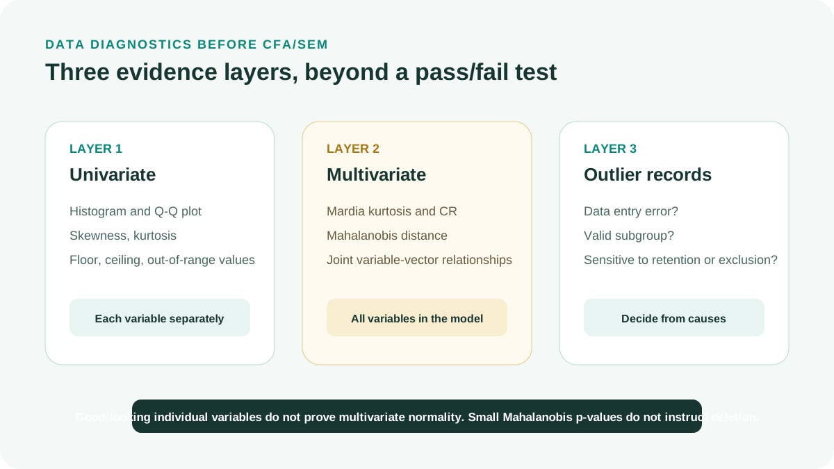
| Layer | Question | Main evidence | Premature conclusion to avoid |
|---|---|---|---|
| Univariate | How skewed or heavy-tailed is each variable? | Histogram, Q-Q plot, skewness, kurtosis | Every variable is approximately normal, so the vector must be normal |
| Multivariate | Does the joint distribution of the variable vector satisfy the assumption? | Mardia-type kurtosis and the AMOS critical ratio | A large critical ratio makes the data unusable |
| Outliers | Which cases are far from the multivariate centroid, and why? | Mahalanobis distance plus original case records | Cases with small p-values must be deleted |
3. Univariate Diagnostics in SPSS
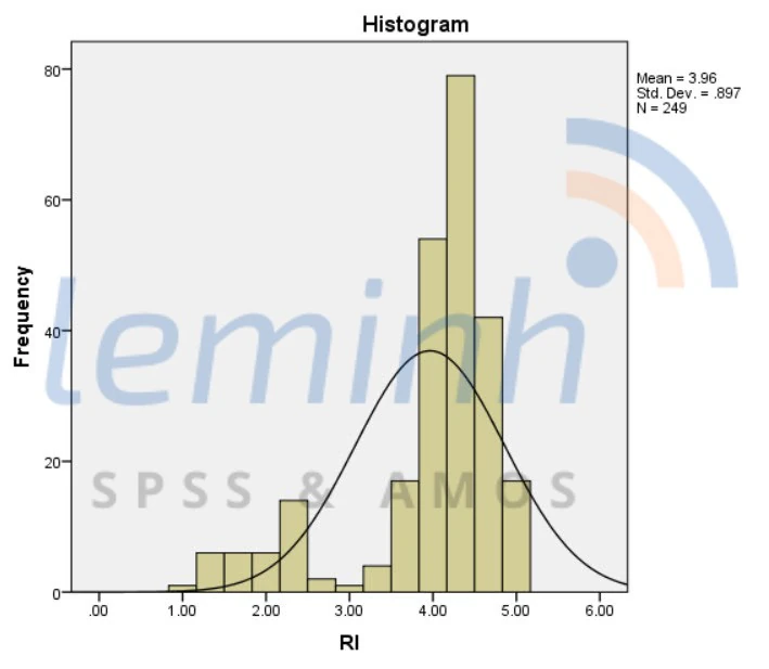
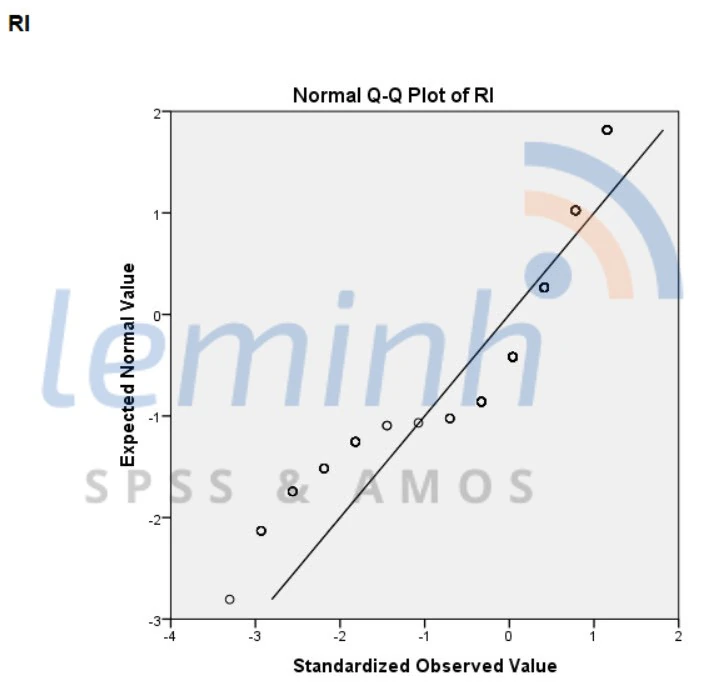
In SPSS, Analyze > Descriptive Statistics > Explore provides histograms, normal Q-Q plots, boxplots, skewness, and kurtosis. Inspect plots before applying thresholds: is there a long tail, bimodality, a ceiling or floor effect, or only mild skewness detectable in a large sample?
Shapiro–Wilk tests exact normality. With large samples, small and practically unimportant deviations can yield p < 0,05. With small samples, the test may lack power. A p-value therefore cannot replace plots, descriptive statistics, and knowledge of the scale.
No pair of skewness and kurtosis cutoffs applies to every design. Kline (2023) notes that some simulation studies treated |skewness| > 2 and |excess kurtosis| > 7 as indications of severe nonnormality, but also emphasizes numerous exceptions and the absence of universal boundaries. Use these benchmarks only as anchors for closer examination rather than automatic rules for estimator selection, transformation, or variable removal.
Open Explore
Place the correct observed variables in Dependent List; use Factor List if group-specific inspection is needed.
Select Plots
Enable histograms and normality plots; retain boxplots to identify cases requiring review.
Read histograms and Q-Q plots
Describe skewness, tails, multiple peaks, and ceiling or floor effects rather than simply stating that normality is met.
Record skewness and kurtosis
Retain SPSS’s reporting convention and do not mix excess kurtosis with Pearson kurtosis.
Check extreme cases
Use case IDs to compare values with questionnaires or the original data source.
Repeat for important groups
For group comparisons, inspect distributions within each group rather than only the pooled sample.
Save output and a log
Record the data version, run date, and every editing decision.

4. Multivariate Normality and Outliers in AMOS
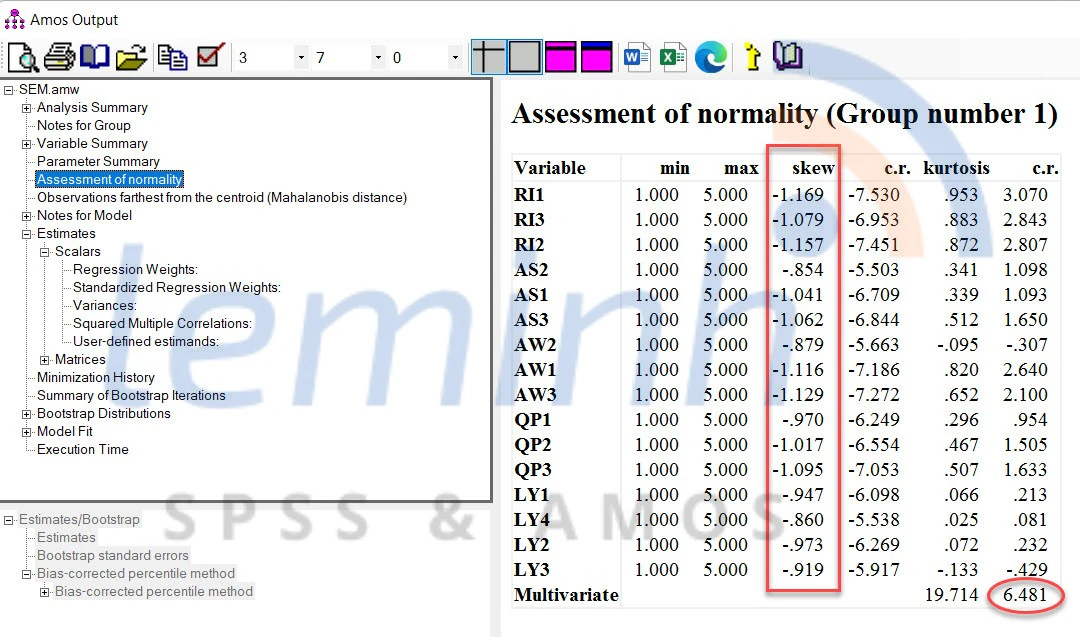
Mardia (1970) developed measures of multivariate skewness and kurtosis. According to IBM Corp. (2022), AMOS provides multivariate kurtosis and its critical ratio in Assessment of normality. This diagnoses the model’s entire variable set rather than averaging univariate kurtoses.
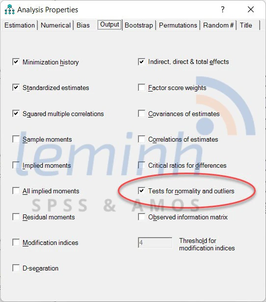
Under Analysis Properties > Output, select Tests for normality and outliers. After estimation, read the individual-variable rows, Multivariate row, and Observations farthest from the centroid table. The critical ratio increases with deviation and sample size, so do not turn a cutoff into an automatic instruction to change estimators.
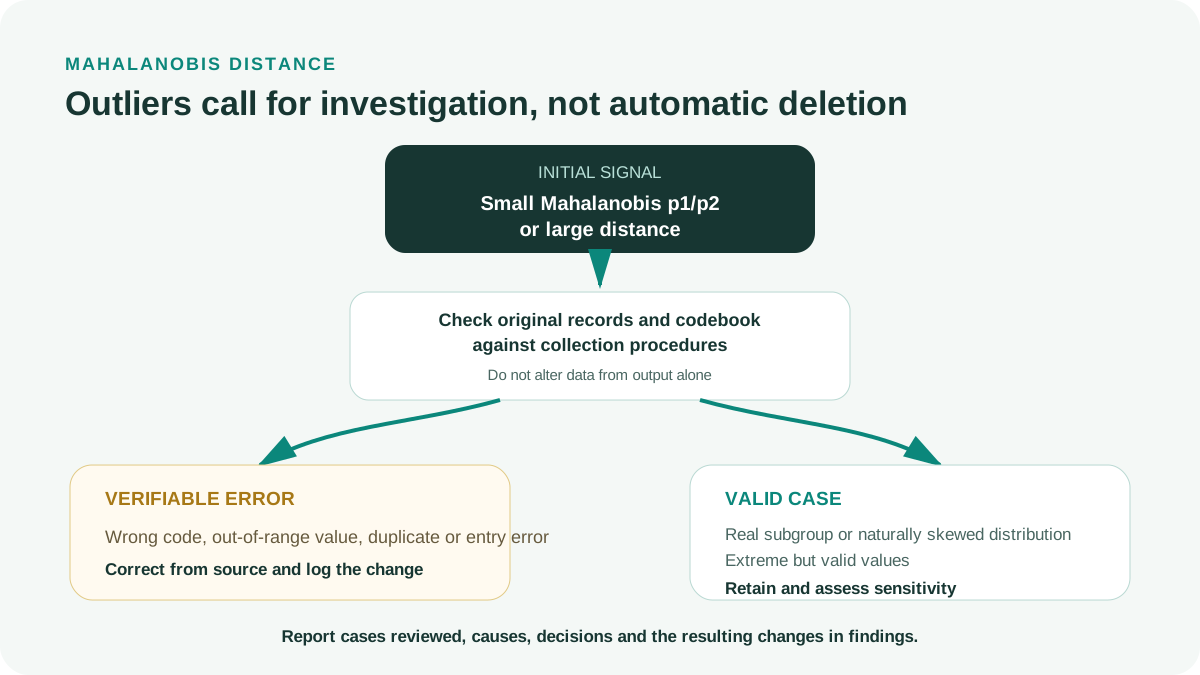
Mahalanobis distance measures multivariate distance from the centroid under the covariance structure. A distant case may reflect an entry error, a valid population member, a subgroup, or a missing structure in the data model. Only original records and the sampling design can distinguish these possibilities.
Enable diagnostics
Under Output, select Tests for normality and outliers before estimation.
Check convergence
Do not interpret diagnostics from a nonconverged model or an inadmissible solution.
Read each variable
Record skewness, kurtosis, and critical ratios as descriptions rather than independent verdicts.
Read the Multivariate row
Record multivariate kurtosis and its critical ratio, and save the variable list used.
Read Mahalanobis distances
Sort the most distant cases and use IDs to return to the original data.
Classify causes
Distinguish data errors, valid cases, subgroups, and coding effects.
Create a sensitivity-analysis version
Where scientifically justified, compare retaining and treating the cases rather than reporting only the favorable version.
5. Handling Outliers Without Overcleaning
Correct entry errors when supported by questionnaires or original sources. Do not replace a valid value with missing solely because it is distant from the center. For valid cases, options include retaining them, using a less sensitive estimator, modeling subgroups, or reporting sensitivity analyses.
Deleting outliers after observing that their removal improves fit is an outcome-dependent decision. This may reduce representativeness and produce overly optimistic reports. If cases are excluded because they fall outside the target population or violate recruitment criteria, apply those criteria consistently.
Winsorization or log transformation can alter a scale’s meaning. Use them only when the transformation suits the variable, is interpretable, and is explicitly documented. Do not transform individual Likert items merely to produce bell-shaped histograms.
| Cause | Main action | Supplementary analysis |
|---|---|---|
| Entry or coding error | Cross-check and correct with an audit trail | Repeat all diagnostics |
| Outside the target population | Apply established exclusion criteria | Report counts and reasons |
| Valid but influential case | Retain in the primary analysis where appropriate | Compare estimates with and without the case |
| Genuine subgroup | Examine sample heterogeneity or multigroup analysis | Assess measurement invariance |
| Naturally skewed distribution | Select an appropriate estimator or CI | Report medians or quantiles when needed |
6. From Diagnostics to Estimator Selection
Ordinary ML may remain useful with modest deviations, sufficient samples, and manageable model complexity, but justify the decision through the sensitivity of standard errors and fit. Robust corrections adjust test statistics or standard errors for nonnormality; they neither change the data nor repair misspecification (Savalei, 2014). Kline (2023) likewise emphasizes assessing assumptions and fit through an evidence profile rather than one cutoff.
AMOS supports bootstrapping and the Bollen–Stine bootstrap. Bollen and Stine (1992) use resampling under the null model to assess overall fit when distributional assumptions are violated. Bootstrap confidence intervals are more suitable for many indirect effects, but bootstrapping does not make data normal.
Severe nonnormality, few-category ordinal data, complex missingness, or requirements for robust standard errors and scaled chi-square may require an estimator in other software. Yuan and Bentler (2000) present likelihood adjustments for nonnormal and missing data; choices must follow the data type and inferential objective.
| Situation | Possible primary analysis | Sensitivity check | Note |
|---|---|---|---|
| Continuous, mildly skewed, adequate sample | ML with complete diagnostics | Bootstrap CIs or a robust estimator | No mechanical transformation needed |
| Clear nonnormality while retaining AMOS | ML plus appropriate bootstrapping | Bollen–Stine and estimate comparisons | State AMOS limitations |
| Few-category ordinal data | Categorical or ordinal estimator | Compare with continuous specification if justified | Do not rely only on skewness |
| Valid influential outlier | Retain in the primary model | Compare with and without the case | Report both if conclusions change |
| Missing data and nonnormality | Estimator directly handling missing data | Specify a plausible missingness mechanism | Avoid arbitrary listwise deletion |
7. Hypothetical Numerical Example: From Diagnostics to Decisions
The following example is illustrative rather than actual research data. A CFA model has 18 Likert items with 5 categories and N = 412. Univariate skewness ranges from -1,18 to 0,74; excess kurtosis ranges from -0,62 to 2,35. Q-Q plots show right tails for three items; AMOS reports a multivariate kurtosis critical ratio of 12,84.
Three observations with Mahalanobis p2 < .001 are investigated. One has a value of 55 on an item ranging from 1 to 5 and is corrected to 5 after checking the questionnaire. The remaining two are valid, very-high-intensity users and are retained.
The team uses ML as the primary model, reports 2.000 bootstrap samples for confidence intervals, and obtains Bollen–Stine p = .074 as supplementary fit evidence. Removing the two valid cases in a sensitivity analysis changes loadings by at most .018 and leaves structural-path conclusions unchanged. Retention therefore has clearer evidential support than mechanical deletion.
| Evidence | Hypothetical result | Interpretation |
|---|---|---|
| Univariate skewness | -1,18 to 0,74 | Moderate skewness in some items |
| Excess kurtosis | -0,62 to 2,35 | Some heavy tails; do not use a cutoff alone |
| Multivariate kurtosis CR | 12,84 | Evidence of multivariate nonnormality |
| Mahalanobis p2 < .001 | 3 cases | One error corrected; two valid cases retained |
| Bollen-Stine p | .074 | Exact fit not rejected under this illustrative procedure |
| Maximum loading change | .018 | Conclusions are relatively insensitive to the two valid cases |
8. Bollen–Stine, Bootstrap Standard Errors, and Robust ML Are Not Interchangeable
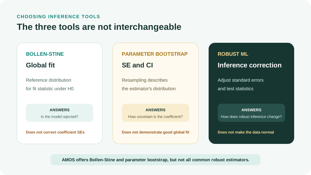
The Bollen–Stine bootstrap generates a reference distribution for the model-fit statistic under the null hypothesis of model correctness. Bollen–Stine p therefore addresses global fit rather than automatically correcting every parameter’s standard error or confidence interval (Bollen and Stine, 1992; Kline, 2023).
Bootstrapping standard errors and confidence intervals is a separate procedure. It resamples to describe the empirical distribution of parameter estimates. If a study requires inference for indirect effects or coefficients with skewed distributions, request bootstrapping for those specific parameters rather than merely enabling Bollen–Stine.
Robust ML retains the basic ML estimates but adjusts standard errors and test statistics for nonnormality. Savalei (2014) shows that robust corrections have multiple forms and assumptions, so reports must name the specific estimator. AMOS does not provide every commonly used robust variant; cross-checking in other software is sometimes necessary.
| Tool | Component addressed | Must not be interpreted as |
|---|---|---|
| Bollen–Stine bootstrap | p-value for global fit | Robust standard errors for all coefficients |
| Parameter bootstrapping | Coefficient standard errors and confidence intervals | The model has good global fit |
| Robust ML | Adjusted standard errors and fit statistics | The data have become normally distributed |
9. Few-Category Likert Data: A Measurement Issue Beyond Normality
Likert items with four or five categories are sometimes treated as approximately continuous when distributions are not extreme and samples are sufficiently large. With two or three categories, severe skewness, or many sparse frequency cells, however, Pearson correlations and ordinary ML may poorly represent relationships between continuous latent variables.
Kline (2023) recommends choosing methods according to measurement level and data conditions. One option is ordinal CFA using polychoric correlations and an estimator such as WLSMV in supporting software. Flora and Curran (2004) show that robust WLS outperforms full WLS in many ordinal-data simulation conditions, particularly with smaller samples; this supports matching estimators to measurement levels rather than applying default ML to every Likert item.
If AMOS with ML is retained, describe it as an approximation, report individual-item distributions, and conduct sensitivity analyses rather than claiming that ML is always robust. AMOS 29 does not offer a categorical estimator equivalent to WLSMV, so ordinal comparisons require supporting software and the same model specification.
| Variable type | Primary analysis to consider | Supplementary check |
|---|---|---|
| Continuous, mildly nonnormal | ML with complete diagnostics | Bootstrapping or a robust estimator |
| Likert with 5 to 7 categories and nonextreme distributions | ML may provide a pragmatic approximation | Compare with ordinal CFA when conclusions are important |
| Binary or 2 to 3 categories | Categorical or ordinal CFA | WLSMV and polychoric or tetrachoric correlations |
| Ceiling effects, floor effects, or very heavy tails | Robust estimator or a distribution-appropriate model | Sensitivity analysis and data checks |
Small skewness does not automatically establish ML’s suitability, and large skewness does not automatically require variable removal. Decisions must consider measurement level, sample, model, and inferential objective.
10. Designing Sensitivity Analyses Before Drawing Conclusions
Sensitivity analysis asks whether scientific conclusions change under another reasonable estimation choice. It provides a practical assessment of nonnormality’s consequences rather than debating whether data are perfectly normal (Yuan and Bentler, 2000; Savalei, 2014).
Do not create dozens of models. Prespecify one primary analysis and one or two comparisons targeting the actual risk: bootstrap parameter confidence intervals, robust ML in other software, ordinal CFA for few-category items, or analyses with and without cases under review.
Step 1
Finalize the primary estimator and its rationale before viewing comparison results.
Step 2
Select a comparison addressing the identified risk rather than one yielding favorable p-values.
Step 3
Compare signs, magnitudes, confidence intervals, and conclusions for focal parameters.
Step 4
Compare global fit without treating small fit differences as the only evidence.
Step 5
Document all sample, variable, missing-data, and estimator changes between runs.
Step 6
If conclusions change, report instability and reduce certainty rather than concealing results.
The primary analysis must still be prespecified. Sensitivity analysis assesses robustness of conclusions rather than providing a reason to change estimators after seeing p-values.
11. Common Interpretation Errors
| Weak practice | Why it is problematic | Remedy |
|---|---|---|
| Shapiro–Wilk p < .05, so SEM is impossible | The test is sensitive to N and considers variables individually | Combine plots, multivariate diagnostics, and estimator choice |
| All skewness values are within ±2, so multivariate normality holds | Univariate normality does not imply multivariate normality | Read the Multivariate row in AMOS |
| A large kurtosis CR requires deleting outliers | It identifies neither cases nor causes | Review Mahalanobis distances and original records |
| Bootstrapping makes the data normal | Bootstrapping changes inference rather than the data | Clearly state the bootstrap objective |
| Bollen–Stine p > .05 proves the model correct | Failure to reject does not confirm theory | Examine fit, residuals, and competing models |
| Delete cases until fit is attractive | Creates outcome-dependent decisions | Establish criteria and report sensitivity analyses |
12. APA 7 Reporting Template and Checklist
The following template uses hypothetical values. Replace bracketed values with actual results; state software versions, bootstrap count, confidence-interval type, and reasons for handling each case.
Example report
Distributions were assessed using histograms and Q-Q plots in SPSS [version], univariate skewness and excess kurtosis, and Tests for normality and outliers in IBM SPSS Amos [version]. Skewness ranged from [min] to [max], excess kurtosis from [min] to [max], and the multivariate kurtosis critical ratio was [ ]. A total of [number] observations were reviewed using Mahalanobis distance; [number] data errors were corrected after cross-checking and [number] valid cases were retained. The primary model was estimated using [estimator]. Given [degree] evidence of nonnormality, the study used [number] bootstrap samples with [type] confidence intervals and Bollen–Stine p = [ ]. Sensitivity analysis [description] indicated [qualified conclusion].
- Check ranges, missing data, and reversed items before normality.
- Distinguish univariate and multivariate normality.
- Inspect histograms and Q-Q plots rather than only p-values.
- State the software’s kurtosis convention.
- Read the Multivariate row in AMOS.
- Trace every large-Mahalanobis-distance case to the original data.
- Do not delete valid cases merely to improve fit.
- Explain the choice of ML, bootstrapping, or a robust estimator.
- Describe the bootstrap count and confidence-interval type.
- Use Bollen–Stine for its intended fit-assessment purpose.
- Conduct sensitivity analysis when decisions may affect results.
- Cross-check every in-text citation against the reference list.
Conclusion
Normality assessment is a diagnostic and decision-making workflow rather than a hunt for p > 0,05. The key questions concern which violations are real, which inferential components are sensitive, and whether conclusions change under reasonable alternatives.
A good report presents the data, causes, estimator, and sensitivity analysis. This protects conclusions more effectively than deleting unusual points or applying one cutoff to every sample.
References
- Bollen, K. A., & Stine, R. A. (1992). Bootstrapping goodness-of-fit measures in structural equation models. Sociological Methods & Research, 21(2), 205-229.https://doi.org/10.1177/0049124192021002004
- Curran, P. J., West, S. G., & Finch, J. F. (1996). The robustness of test statistics to nonnormality and specification error in confirmatory factor analysis. Psychological Methods, 1(1), 16-29.https://doi.org/10.1037/1082-989X.1.1.16
- Mardia, K. V. (1970). Measures of multivariate skewness and kurtosis with applications. Biometrika, 57(3), 519-530.https://doi.org/10.1093/biomet/57.3.519
- Savalei, V. (2014). Understanding robust corrections in structural equation modeling. Structural Equation Modeling: A Multidisciplinary Journal, 21(1), 149-160.https://doi.org/10.1080/10705511.2013.824793
- Yuan, K. H., & Bentler, P. M. (2000). Three likelihood-based methods for mean and covariance structure analysis with nonnormal missing data. Sociological Methodology, 30(1), 165-200.https://doi.org/10.1111/0081-1750.00078
- Flora, D. B., & Curran, P. J. (2004). An empirical evaluation of alternative methods of estimation for confirmatory factor analysis with ordinal data. Psychological Methods, 9(4), 466-491.https://doi.org/10.1037/1082-989X.9.4.466
- IBM Corp. (2022). IBM SPSS Amos 29 user's guide.https://www.ibm.com/docs/en/SSLVMB_29.0.0/pdf/IBM_SPSS_Amos_User_Guide.pdf
- Kline, R. B. (2023). Principles and practice of structural equation modeling (5th ed.). Guilford Press.https://www.guilford.com/books/Principles-and-Practice-of-Structural-Equation-Modeling/Rex-Kline/9781462551910
Academic note: The example values are hypothetical and illustrate the workflow. Few-category ordinal data, severe nonnormality, or complex missingness may require another estimator and software rather than default ML in AMOS.