
fsQCA from Calibration to Solutions: An Auditable Practical Workflow
fsQCA examines combinations of conditions associated with an outcome rather than ranking isolated variable effects. An auditable analysis explains set meaning, calibration anchors, truth-table decisions and the counterfactual assumptions used to simplify solutions.
Define sets before calibration, distinguish necessity from sufficiency and read consistency alongside coverage. Retain simplification assumptions and assess sensitivity. Observed configurations do not independently establish causation, and coverage is not R².
fsQCA: from sets to outcome configurations
- Calibration
Justify set-membership anchors
- Truth table
Review frequency and consistency
- Solutions
Interpret alternative configurations
- Robustness
Check sensitivity and report choices
Conceptual diagram. Do not interpret an fsQCA configuration as a net-effect coefficient.
Source: Lê Minh · Conceptual illustration, not software output.1. Ask about combinations rather than isolated variables
Whether digital capability relates to performance is different from asking which combinations of capability, support and resources are associated with high performance. fsQCA addresses the configurational question, allowing alternative paths to the same outcome and causal asymmetry. The explanation of a low outcome need not be the inverse of the explanation of a high outcome (Ragin, 2008, Chapters 1–2).
Membership from 0 to 1 indicates how strongly a case belongs to a substantively defined set. A score of .8 in the set of strongly supported organizations is not an 80% probability. Exactly .5 marks maximum ambiguity about being more in or more out of the set (Ragin, 2008, Chapters 2, 5).
For the usual fuzzy-set operations, ~A = 1 − A, A*B = min(A,B), and A+B = max(A,B). Negation, intersection and union operate on calibrated membership, not directly on raw 1–5 Likert codes (Ragin, 2008, Chapter 2).
| Statement | Meaning under investigation | What does not follow |
|---|---|---|
| A*B → Y | A and B together are sufficient for Y | A or B alone is sufficient |
| Y → A | A is necessary for Y | A guarantees Y |
| A*B + C → Y | Alternative paths: A with B, or C | The paths do not overlap |
| ~Y | The negated outcome, requiring its own analysis | Reverse every sign in the solution for Y |
2. Prepare the file and define the target sets
Use one case per row within a coherent study scope and retain an ID for case-level review. Record original variables, scale-scoring rules, reverse coding and missing-data handling. If input scores are item means, say so. If they are exported PLS-SEM construct scores, identify the model and export procedure; these scoring methods are not automatically interchangeable.
For each set, record its name, substantive meaning of strong membership and nonmembership, measurement unit and anchor rationale. Sufficient resources for a particular project is more specific than high resources without a reference standard. Substantive definition precedes numerical transformation (Ragin, 2008, Chapters 4–5).
Choose conditions from theory and case knowledge. A truth table with k conditions has 2^k possible rows: six conditions produce 64 combinations. Adding conditions to obtain attractive findings increases the configuration space and the risk of limited diversity, where many combinations lack observed cases (Ragin, 2008, Chapters 7–8).
- Keep IDs and original data separate from calibrated columns.
- Specify input scoring, reverse items and missing-data rules.
- Define the outcome and every condition set.
- Record the software and version actually used.
- Do not add conditions solely in response to a preferred solution.
3. Three anchors are not three compulsory percentiles
Direct calibration uses qualitative anchors for full nonmembership, the crossover and full membership. Ragin's (2008, Chapter 5) presentation commonly associates them with approximately .05, .50 and .95 membership. These are membership values, not a requirement to use the 5th, 50th and 95th percentiles of every input distribution.
Constructed example: a 1–7 mean scale represents strong support. Anchors at 2, 4 and 6 may be an illustrative specification only if response meanings and contextual knowledge justify them. They are not general recommendations for seven-point scales. Explain why 4 distinguishes the two sides of the set instead of relying on its arithmetic midpoint (Ragin, 2008, Chapters 4–5).
Percentiles may inform a justified specification when external standards are unavailable, but they make set meaning sample-dependent. Report percentile choices, corresponding raw values and defensible alternatives. Simple min–max normalization is not automatically substantive set calibration (Ragin, 2008, Chapters 4–5).
After calibration, inspect both sides of .5, cases exactly at .5, missing codes, bounds and typical cases. Do not add an unexplained constant to avoid crossover cases. Record any adjustment, affected cases and sensitivity results.
| Field | Required information |
|---|---|
| Target set | Meaning of strong membership and nonmembership |
| Input | Raw variable, item mean or construct score, with units |
| Anchors | Full-out, crossover, full-in and reasons |
| Checks | Distribution, missingness, crossover cases and typical cases |
| Sensitivity | Defensible alternative anchors and resulting changes |
Each change needs a substantive reason or an explicitly documented sensitivity purpose. Do not repeatedly change anchors until a desired consistency or coverage appears and publish only that specification.
4. Necessity, sufficiency and the denominator
For C to be sufficient for Y, membership in C should not exceed membership in Y. Sufficiency consistency assesses compatibility with that subset relation; coverage assesses how much outcome membership is covered. The formulas share a numerator but use different denominators. Neither measure is a p-value or R² (Ragin, 2008, pp. 52–55).
Necessity reverses the subset relation: Y should be a subset of A. Its consistency denominator is total membership in Y. A condition present almost everywhere may have high necessity consistency but little discriminatory value. Examine coverage, prevalence and substantive relevance as well (Ragin, 2008, pp. 53–63).
Assess necessity separately, examine plots and contradictory cases, and retain theoretically justified negations (Ragin, 2008, Chapter 3). Causal claims still require theory, temporal ordering and case knowledge.
Cons_suff(C → Y) = sum(min(C_i, Y_i)) / sum(C_i)
Cov_suff(C → Y)  = sum(min(C_i, Y_i)) / sum(Y_i)
Cons_nec(Y → A)  = sum(min(A_i, Y_i)) / sum(Y_i)
Cov_nec(Y → A)   = sum(min(A_i, Y_i)) / sum(A_i)
Ratios require positive denominators.
5. A small worked calculation
The four cases below are constructed to check formulas, not to support a substantive solution. For C = A*B, the rowwise minima are .7, .6, .3 and .2. Total C is 1.8, total Y is 1.9, and total min(C,Y) is 1.6.
Sufficiency consistency is 1.6/1.8 = .889 and coverage is 1.6/1.9 = .842. They differ because they answer different questions. For the necessity of A, total min(A,Y) is 1.8, giving 1.8/1.9 = .947. That necessity result cannot establish the sufficiency of A (formulas from Ragin, 2008, Chapter 3).
| Case | A | B | Y | C = min(A,B) | min(C,Y) |
|---|---|---|---|---|---|
| 1 | .8 | .7 | .9 | .7 | .7 |
| 2 | .6 | .9 | .5 | .6 | .5 |
| 3 | .4 | .3 | .4 | .3 | .3 |
| 4 | .2 | .8 | .1 | .2 | .1 |
A <- c(.8, .6, .4, .2)
B <- c(.7, .9, .3, .8)
Y <- c(.9, .5, .4, .1)
C <- pmin(A, B)
stopifnot(sum(C) > 0, sum(Y) > 0)
c(cons_suff = sum(pmin(C,Y))/sum(C),
  cov_suff = sum(pmin(C,Y))/sum(Y),
  cons_nec_A = sum(pmin(A,Y))/sum(Y))
# 0.8888889, 0.8421053, 0.9473684
6. From the input file to the truth table
The workflow specifies reproducible decisions rather than assuming a button layout shared by all versions. Record the application, create separate calibrated variables and inspect the named outputs. Truth-table and minimization logic follow Ragin (2008, Chapters 7–9).
Keep frequency, consistency and PRI distinct. Frequency counts cases above .5 membership in a configuration; PRI is an alternative consistency measure based on a reduction-in-error calculation. Retain settings, reasons and row decisions (Ragin, 2017, pp. 52–54).
For fsQCA 3.0 as documented in the manual, Compute uses calibrate(x,n1,n2,n3) in full-in, crossover, full-out order. Constructed example: calibrate(SUPPORT,6,4,2). Open Analyze > Truth Table Algorithm for the table. Check your installed version before following menu paths (Ragin, 2017, pp. 14–15, 51–52).
Import and inspect
Check IDs, case counts, variable types, missingness, reverse coding and score construction. Preserve the link to the original model when using PLS scores.
Create calibrated sets
Enter justified anchors and keep raw columns. Inspect membership bounds, endpoints and crossover cases; stop if coding or set direction is wrong.
Examine necessity
Assess justified conditions and negations with consistency, coverage and case plots. Do not report these as sufficient configurations.
Construct the truth table
Select the specified outcome and conditions. Inspect row frequencies, consistency, PRI, unobserved combinations and contradictory rows.
Document row decisions
Justify cutoffs using the design, case count, distribution and substantive knowledge. Save both the full and analysis-ready truth table.
Minimize transparently
Distinguish complex, parsimonious and intermediate solutions. Retain directional expectations and simplification assumptions.
Return to cases
Inspect configuration consistency, raw and unique coverage and plots. Trace typical or contradictory cases to IDs.
Assess negation and sensitivity
Analyze ~Y separately when required. Document defensible anchor or cutoff alternatives; use holdout assessment only when the design and sample permit it.
7. Solution types and counterfactual assumptions
An unobserved truth-table row is a logical remainder, not a combination shown to produce a low outcome. Complex solutions do not use remainders for simplification. Parsimonious solutions allow simplifying remainders, potentially including substantively difficult assumptions. Intermediate solutions constrain assumptions using justified directional expectations (Ragin, 2008, Chapters 8–9).
A shorter solution is not necessarily more defensible. Identify which conditions disappear through assumptions about unobserved situations. Do not choose directional expectations after inspecting solutions to obtain a preferred configuration. If several solution models are produced, retain them and justify the model used (Ragin, 2008, Chapter 9).
Any core/peripheral classification requires an explicit comparison rule across solutions under the same specification. It cannot be inferred from circle size, regression beta or raw coverage alone. When a supplied figure only distinguishes presence and absence, preserve that reporting limit.
| Solution | Required record |
|---|---|
| Complex | Included observed rows without remainder-based simplification |
| Parsimonious | Simplifying assumptions and substantive plausibility |
| Intermediate | Directional expectations and accepted counterfactuals |
| Multiple solution models | Available alternatives and the reason for the model reported |
8. Read the supplied fIIP and fIWP configuration tables
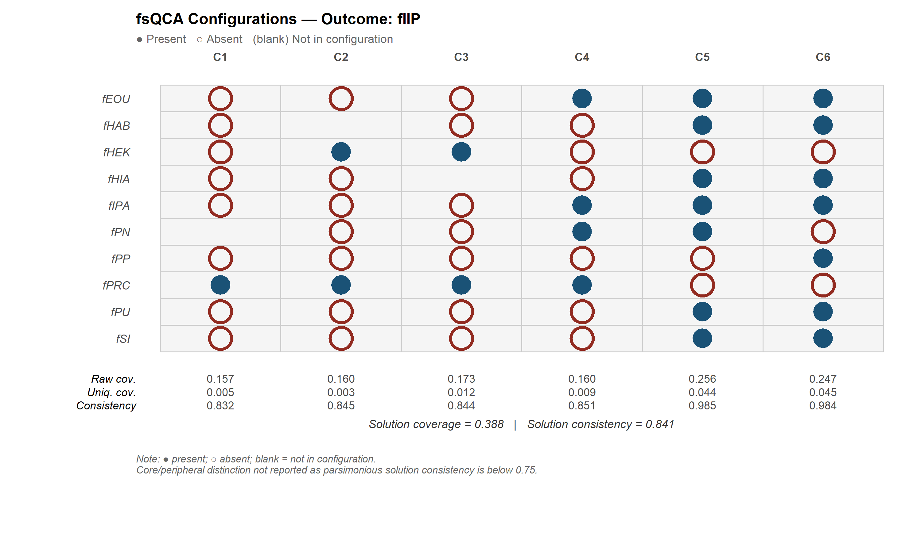
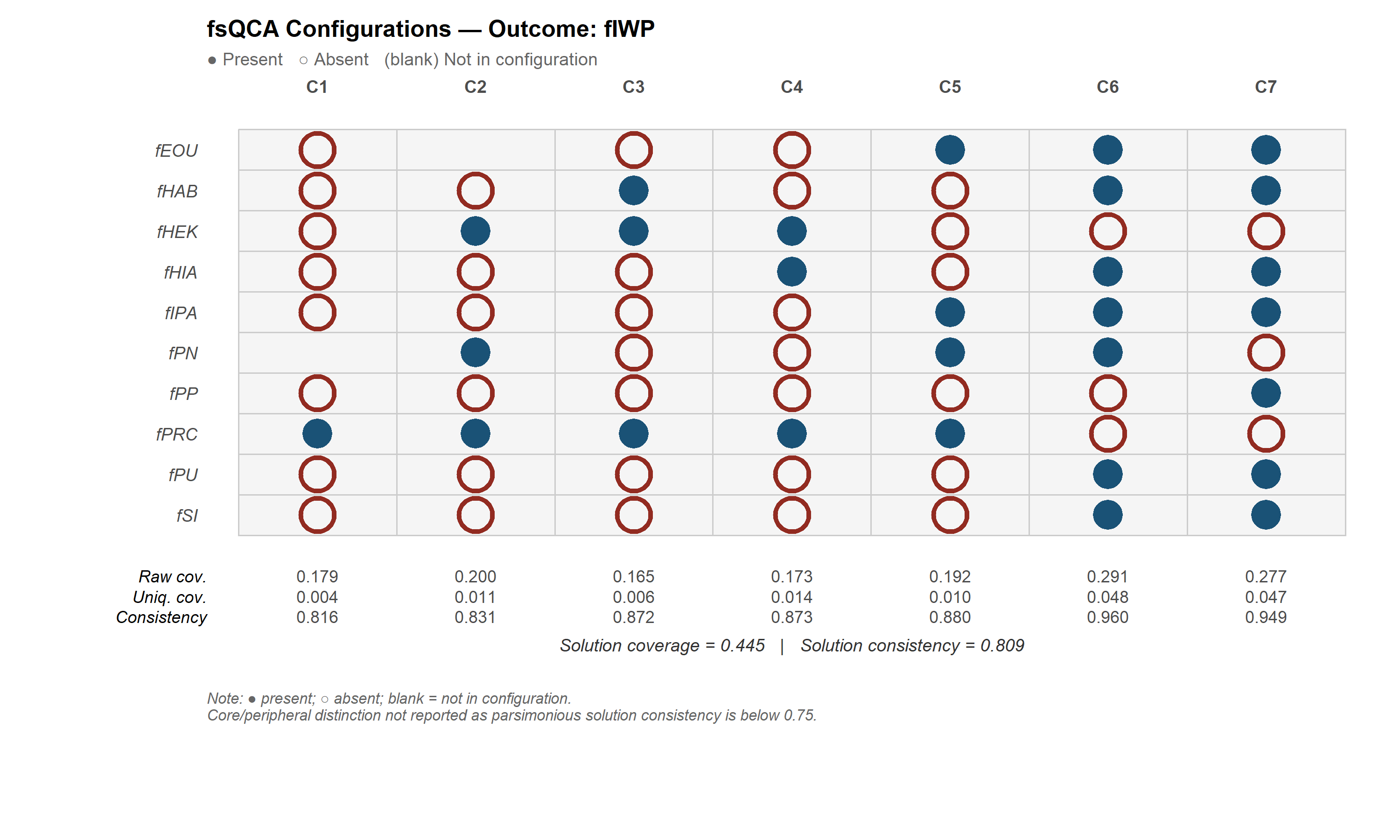
The two figures supplied by Lê Minh contain six fIIP and seven fIWP configurations. They support learning to read a configuration table, not certification of the underlying dataset. Each column is a configuration: a filled circle indicates presence, an open circle indicates negation, and a blank indicates an omitted condition. A blank is not missing data; an open circle is not a negative regression coefficient.
In fIIP, C1 has raw coverage .157, unique coverage .005 and consistency .832. Raw coverage includes overlap with other paths; unique coverage is the part attributable only to that path within the reported solution. Because paths overlap, their raw coverages must not be added to obtain solution coverage (Ragin, 2008, pp. 64–67).
The fIIP solution has coverage .388 and consistency .841; fIWP has .445 and .809. Do not call these 38.8% and 44.5% explained variance. Higher coverage alone does not establish that fIWP has a better solution: the outcomes differ and consistency differs too. Calibration, truth tables and case information are needed for substantive assessment.
The figures state that core/peripheral roles are not distinguished in this example. Their note mentioning .75 is not a universal decision rule. A thesis should also supply a codebook for fEOU, fHAB and the other set labels; their meanings are not guessed here.
Reporting template
Template to complete with actual findings: Sets [names and definitions] were calibrated using [method] and anchors [full-out/crossover/full-in], justified by [evidence]. Necessity was assessed separately. The truth table used frequency [ ], consistency [ ] and PRI [ ], with reasons [ ]. The [type] solution contained [ ] configurations; directional expectations and simplifying assumptions were [ ]. Solution consistency was [ ] and coverage [ ]. Sensitivity checks of [anchors/cutoffs/cases/negated outcome] showed [specific stability or sensitivity]. Findings were interpreted as set relations within the study scope.
9. Sensitivity and reasons to pause strong conclusions
Compare the original specification with each defensible alternative. Track condition membership in solutions, disappearing configurations, consistency, coverage and typical or contradictory cases. Exact symbolic identity is not the only stability criterion, but a central conclusion that changes under a small justified anchor adjustment must be reported as sensitive.
Pause strong conclusions when anchors lack justification, apparent sufficiency for both Y and ~Y is unexplained, empirical support is weak across many combinations or unusual cases cannot be traced. These are reasons to review the design, not silently delete observations.
Pappas and Woodside (2021) encourage contrarian-case analysis and predictive checks. If an independent or suitable holdout sample is available, evaluate rules fixed in the development sample. Analysis of the pooled sample must not be labelled out-of-sample validation. Stability still requires bounded inference and contextual evidence.
- Explain sets, input scoring and anchors.
- Retain raw data, membership and IDs under controlled access.
- Separate necessity and sufficiency results.
- Keep full truth tables, cutoffs and row decisions.
- Report solution types, expectations and simplification assumptions.
- Report configuration and solution consistency/coverage.
- Do not sum raw coverage or call coverage R².
- Analyze ~Y and sensitivity where the question requires them.
- Retain inconvenient findings; protect identifying information.
Conclusion
A defensible fsQCA report lets readers trace set definitions through membership scores and truth-table choices to the final solutions. The configuration table presents the result; calibration reasons, counterfactual assumptions and case knowledge make that result interpretable.
References
- Ragin, C. C. (2008). Redesigning social inquiry: Fuzzy sets and beyond. University of Chicago Press. Chapters 2–5, 7–9. https://press.uchicago.edu/ucp/books/book/chicago/R/bo5973952.html
- Pappas, I. O., & Woodside, A. G. (2021). Fuzzy-set Qualitative Comparative Analysis (fsQCA): Guidelines for research practice in Information Systems and marketing. International Journal of Information Management, 58, 102310. https://doi.org/10.1016/j.ijinfomgt.2021.102310
- Ragin, C. C. (2017). User’s guide to Fuzzy-Set / Qualitative Comparative Analysis (fsQCA 3.0). University of California, Irvine. https://sites.socsci.uci.edu/~cragin/fsQCA/download/fsQCAManual.pdf
Methodological note: Small numerical examples are constructed for teaching and are separate from owner-supplied fIIP/fIWP figures. Formulas and set-theoretic reasoning were checked against Ragin (2008). Cutoffs need design-specific justification rather than treatment as universal standards.