EFA of Likert Data Using SPSS, R, and FACTOR: A Reproducible Workflow

SPSS is convenient for Pearson-based EFA, but few-category or strongly skewed Likert data may require polychoric correlations and ordinal parallel analysis. This guide places three programs within one decision workflow.

EFA, LIKERT DATA AND SOFTWAREPrepared by Lê Minh10 minUpdated 29/10/2026

KEY ARGUMENT

Choose among SPSS, R and FACTOR; inspect data, select correlations, determine factor count, extract and rotate, address warnings, compare sensitivity solutions and report reproducibly.

Start reading

1. Objectives and input data

This workflow explores scale structure from Likert items. Use rectangular data with respondents in rows and items in columns; the codebook must identify reversed items, missing values and valid ranges.

EFA does not replace theory. Map each item to its expected construct and content domain before analysis. Software examines column relationships without knowing substantive importance (Fabrigar & Wegener, 2012; Finch et al., 2016).

Provide a codebook and reverse-coding rules.
Give each item a brief content label.
Identify ordinal or approximately continuous treatment.
Reserve CFA data or plan independent confirmation.
Do not combine unrelated instruments merely because they share a file.

2. Software decision map

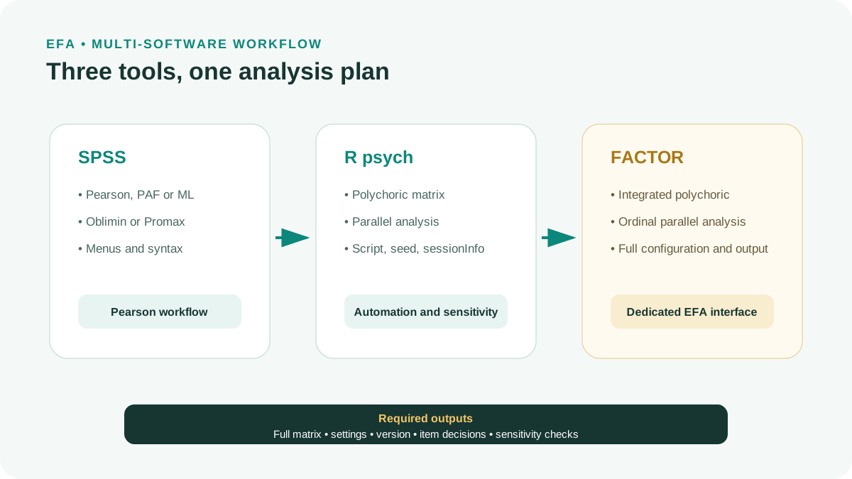
No program is best for every situation. SPSS suits Pearson, PAF and oblique rotation; R supports automation and specification comparisons; FACTOR offers polychoric correlations and parallel analysis in a dedicated EFA tool (Lorenzo-Seva & Ferrando, 2006).

Roles of SPSS, R psych and FACTOR in EFA — The tools address different needs, but each must preserve assessable settings, versions and decisions.

Table 1
Need	SPSS	R psych	FACTOR
Menu-based Pearson EFA	Very suitable	Available	Available
Polychoric	Not in the default FACTOR dialog	Yes	Yes
Parallel analysis ordinal	Requires an additional workflow	Yes	Yes
Reproducible scripting	Syntax	R script	Configuration and output files
Beginners with little coding experience	Easy	Requires learning commands	Accessible interface

3. Step 1: clean and check coding

Tabulate each item. Find out-of-range values, zero-variance variables, unreversed items, sparse categories and numeric missing codes such as 99. Unreversed items can generate negative loadings or artificial factors.

Specify missing-data treatment before EFA. Listwise deletion reduces N and can change sample composition. Do not automatically mean-impute each item because variance and correlations can shrink.

All item responses lie within valid ranges.
Reverse-coding formulas are documented.
Missing codes are not treated as responses.
Record the remaining sample size.
Check almost identically worded pairs.

4. Step 2: choose Pearson or polychoric correlations

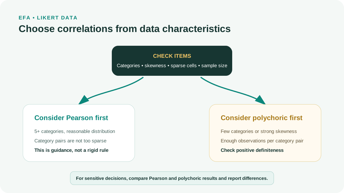
Pearson may be defensible with at least five categories, moderate distributions and reasonably populated response pairs (Rhemtulla et al., 2012). Polychoric correlations model continuous latent variables categorized into ordinal responses; consider them with fewer or concentrated categories (Flora & Curran, 2004; Watkins, 2018).

Polychoric is not automatically superior. With small N and many 0 cross-tabulation cells, estimates can be unstable or the matrix non-positive-definite. Comparing Pearson and polychoric sensitivity is often more useful than one slogan for all Likert data.

Choosing Pearson or polychoric correlations for Likert EFA — Category count, distribution and sparse response pairs jointly inform matrix selection; sensitivity checks help when the choice is uncertain.

Table 2
Signal	Priority consideration	Caution
5-7 categories, reasonably balanced distributions	Pearson	Still assess sensitivity for consequential decisions
2-4 categories or strong skewness	Polychoric	Requires enough observations in category pairs
Many empty cells	Justified category collapsing or increased sample	Do not collapse merely to force estimation
Solutions differ across matrices	Report both	Do not select the favorable result without explanation

5. Step 3: parallel analysis for factor retention

Do not rely only on eigenvalue > 1. Parallel analysis compares observed eigenvalues with random-data distributions. MAP and scree add evidence; final factors must remain interpretable with enough quality items (O'Connor, 2000; Watkins, 2018).

For ordinal data, use parallel analysis appropriate to the polychoric matrix. Garrido et al. (2013) demonstrate ordinal influences on retention. Record reference-data generation, repetitions and percentiles where supported.

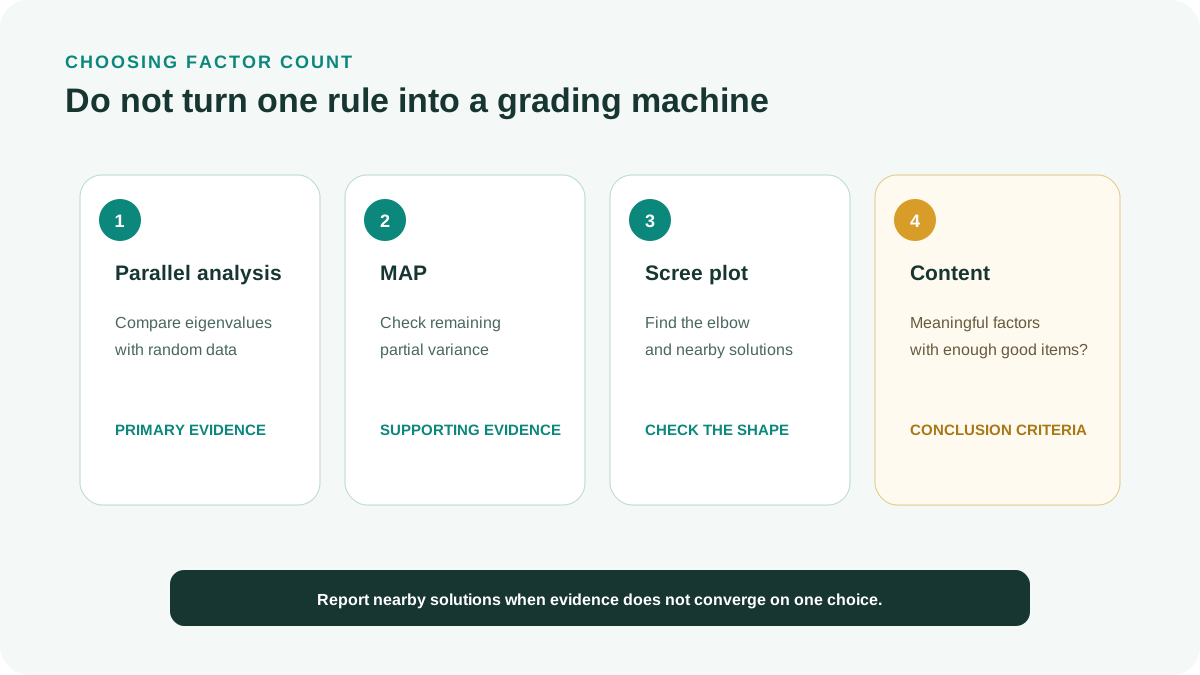
Four evidence layers for factor retention in EFA — Parallel analysis is primary evidence, complemented by MAP, scree and substantive interpretation.

Do not select factor count after viewing loadings and call it confirmation

Comparing neighboring solutions is valid when transparent. Trying many and reporting only the most attractive introduces favorable post-data selection.

6. Step 4A: EFA in SPSS

IBM describes PAF, ML and oblique rotations in Factor, but FACTOR defaults to PCA and Varimax unless specified otherwise (IBM, n.d.). Do not simply accept every default.

Open Factor

Choose Analyze > Dimension Reduction > Factor and add shared-domain items to Variables.

Select Descriptives

Request KMO and Bartlett, anti-image and reproduced correlations.

Select Extraction

Change Principal Components to Principal Axis Factoring and request a scree plot.

Enter the factor count

Set Fixed number of factors from parallel analysis and theory.

Select Rotation

Use Direct Oblimin or Promax when factors may correlate.

Inspect all relevant output

Read communalities, pattern, structure, factor correlations and residuals.

Save syntax

Choose Paste before Run to preserve a reproducible specification.

7. Step 4B: ordinal EFA in R

A minimal workflow reads data, selects items, checks frequencies, computes polychoric correlations, runs parallel analysis and fits fa with the chosen factor count. Set a seed for simulation and preserve sessionInfo to document R/package versions.

Function names can change. psych documents polychoric, fa.parallel and fa; consult help for your installed version rather than copying unchecked code (Revelle, 2026).

Reporting example in English

items <- dat[c('q1','q2','q3','q4','q5','q6')] poly <- psych::polychoric(items)$rho set.seed(20261023) psych::fa.parallel(poly, n.obs = nrow(items), fa = 'fa') fit <- psych::fa(poly, nfactors = 2, n.obs = nrow(items), fm = 'minres', rotate = 'oblimin') print(fit$loadings, cutoff = 0) fit$Phi

8. Step 4C: EFA in FACTOR

Import data and identify ordinal items. Select polychoric correlations, parallel analysis and a common-factor estimator. Use oblique rotation for related constructs. Export full output and configuration rather than just a loading screenshot.

FACTOR brings procedures such as polychoric correlations and parallel analysis into practical EFA (Lorenzo-Seva & Ferrando, 2006). Check the current manual because menus can change.

Use correct decimal and missing-value formats.
Specify each item’s category count.
Match parallel analysis to the data type.
Record estimator and rotation.
Investigate matrix or Heywood warnings.

9. Step 5: read output in a consistent order

Inspect factor count and convergence first, then communalities, pattern, factor correlations and residuals. With oblique rotation, structure does not replace pattern because it also reflects factor correlations (Finch et al., 2016).

Name factors from shared content across strong items, not one standout item. A factor dominated by reversed or similarly worded items may reflect a method effect.

Table 3
Table	Question	Signal to investigate
Parallel analysis	How many factors?	Borderline or theoretically inconsistent solution
Communalities	How much item variance is explained?	Many very low communalities
Pattern matrix	Which factor uniquely relates to each item?	Low loadings or cross-loadings
Factor correlations	How distinct are factors?	Excessive correlations
Residuals	How well are correlations reproduced?	Many large residuals

10. Step 6: warnings and improper solutions

Table 4
Warning	Possible cause	Action
Correlation matrix not positive definite	Duplicate items, unstable polychoric estimates or sparse cells	Inspect eigenvalues, item pairs and frequencies
Heywood case	Communality > 1 or negative uniqueness	Review factors, items, estimator and N
Nonconvergence	Excessive complexity or weak data	Justify simplification rather than only increasing iterations
Factor with 1-2 items	Insufficient substantive identification	Develop items or reconsider factor count
Sign-reversed solution	Factor sign indeterminacy	A complete sign reversal need not change meaning

11. Step 7: sensitivity across specifications

Prespecify primary and sensitivity analyses. For example, primary polychoric/MINRES/oblimin versus sensitivity Pearson/PAF/Promax. Compare factors, item membership, primary loadings and factor correlations.

Similar structures strengthen stability. Investigate differences through skewed items, sparse cells or estimators. Sensitivity is not unlimited searching for the desired result.

Primary analysis, sensitivity and decision rule

Choose the primary analysis from the data type before estimation. Sensitivity examines assumption dependence. The decision rule identifies differences that would change conclusions.

12. Hypothetical example: three programs, one decision

These values are illustrative. A set of 15 four-category Likert items has N = 360, with four strongly skewed items. Pearson parallel analysis suggests four factors, polychoric suggests three, and scree/content support three.

SPSS Pearson/PAF/Promax gives Q09 loadings 0.41 on F2 and 0.38 on F3. R and FACTOR polychoric give Q09 loadings 0.52 on F2 and 0.20 on F3. Item review suggests rare responses attenuate Pearson correlations. The primary ordinal analysis retains Q09 and reports the sensitivity finding.

Table 5
Specification	Factor count	Q09	Decision
SPSS Pearson, PAF, Promax	4 from Pearson PA; also compare 3	0,41 / 0,38	Sensitive to correlation matrix
R polychoric, MINRES, oblimin	3	0,52 / 0,20	Retain in primary analysis
FACTOR polychoric	3	Close to R solution	Supports reproducibility

13. Eight common mistakes

Table 6
Mistake	Consequence	Correction
Accepting SPSS defaults	Unintended PCA and Varimax	Specify PAF/ML and rotation
Using only KMO/Bartlett	Cannot determine factor count	Add PA, MAP, scree and theory
Treating every Likert item as continuous	Ignores ordinal measurement and skewness	Inspect categories, distributions and sparsity
Unchecked polychoric estimation	Unstable matrix	Inspect warnings and sensitivity
Hiding small loadings	Conceals cross-loadings	Preserve the complete matrix
Saving only screenshots	Not reproducible	Save syntax, scripts, configurations and versions
Deleting many items together	Cannot identify what changed the solution	One item per iteration
CFA immediately on the same sample	Overoptimistic fit	Reserve confirmation data

14. APA 7 reporting template and checklist

Reporting example in English

EFA analyzed [n] observations and [p] [category-count] items. Primary analysis used [Pearson/polychoric], [estimator/extraction] and [rotation]. Factors were retained using parallel analysis [details], scree and content. Sensitivity analysis with [specification] yielded [similar/different] results. Final pattern loadings were [range], communalities [range] and factor correlations [range]. Analyses used [software/version]; scripts and output were stored at [ ].

Describe coding and missing-data treatment.
Report item categories and distributions.
Identify Pearson or polychoric correlations.
Report software and versions.
Describe parallel analysis and settings.
State estimator or extraction.
State rotation.
Report the full pattern matrix.
Report factor correlations.
Describe warnings and responses.
Distinguish primary and sensitivity analyses.
Record removed or rewritten items.
Do not make cutoffs absolute rules.
Save syntax, seed and session information.
Use CFA or independent data for confirmation.

Conclusion

The important differences concern correlations, retention and reproducibility rather than software logos. SPSS, R and FACTOR complement each other when following a prespecified plan.

Let Likert data characteristics determine the primary analysis and use sensitivity to assess conclusions. Do not choose software or solutions merely for attractive loadings.

References

Fabrigar, L. R., & Wegener, D. T. (2012). Exploratory factor analysis. Oxford University Press.https://doi.org/10.1093/acprof:osobl/9780199734177.001.0001
Finch, W. H., Immekus, J. C., & French, B. F. (2016). Applied psychometrics using SPSS and AMOS. Information Age Publishing.https://www.infoagepub.com/products/Applied-Psychometrics-using-SPSS-and-AMOS
Flora, D. B., & Curran, P. J. (2004). An empirical evaluation of alternative methods of estimation for confirmatory factor analysis with ordinal data. Psychological Methods, 9(4), 466-491.https://doi.org/10.1037/1082-989X.9.4.466
Garrido, L. E., Abad, F. J., & Ponsoda, V. (2013). A new look at Horn's parallel analysis with ordinal variables. Psychological Methods, 18(4), 454-474.https://doi.org/10.1037/a0030005
IBM. (n.d.). Factor analysis extraction.https://www.ibm.com/docs/en/spss-statistics/31.0.0?topic=analysis-factor-extraction
Lorenzo-Seva, U., & Ferrando, P. J. (2006). FACTOR: A computer program to fit the exploratory factor analysis model. Behavior Research Methods, 38, 88-91.https://doi.org/10.3758/BF03192753
O'Connor, B. P. (2000). SPSS and SAS programs for determining the number of components using parallel analysis and Velicer's MAP test. Behavior Research Methods, Instruments, & Computers, 32(3), 396-402.https://doi.org/10.3758/BF03200807
Revelle, W. (2026). psych: Procedures for psychological, psychometric, and personality research.https://cran.r-project.org/package=psych
Rhemtulla, M., Brosseau-Liard, P. É., & Savalei, V. (2012). When can categorical variables be treated as continuous? A comparison of robust continuous and categorical SEM estimation methods under suboptimal conditions. Psychological Methods, 17(3), 354-373.https://doi.org/10.1037/a0029315
Watkins, M. W. (2018). Exploratory factor analysis: A guide to best practice. Journal of Black Psychology, 44(3), 219-246.https://doi.org/10.1177/0095798418771807

Methodological note: Menus and defaults can change between versions. Consult the current manual and preserve complete settings for reproduction.