
GoF, R², f², and Prediction in SmartPLS 4: Current Approaches to Model Evaluation
GoF was once used as an overall PLS-SEM index, but it cannot reliably distinguish correctly from incorrectly specified models. Reporting should separate in-sample explanation from out-of-sample prediction.
Do not use GoF to establish PLS-SEM model fit. Assess measurement first, then interpret path coefficients, confidence intervals, R², f², PLSpredict and CVPAT according to the question each answers.
1. What was GoF designed to do?
GoF was developed to combine measurement quality with the explanatory power of the structural model. Its usual formula is the square root of average communality multiplied by average R². Originally it was intended to provide an overall view of a PLS path model (Tenenhaus et al., 2005).
Its diagnostic performance is the problem. Simulations by Henseler and Sarstedt (2013) showed that GoF and relative GoF are unsuitable for model validation because they do not consistently distinguish correct from misspecified models. SmartPLS also advises against GoF as an overall fit measure (SmartPLS, n.d.-a).
The values 0.10, 0.25 and 0.36 have been labeled small, medium and large. These benchmarks do not resolve the index’s diagnostic limitations. High GoF can accompany problematic measurement or misspecified structural paths.
Do not write: “GoF = 0.42, therefore the model fits well.” This value is insufficient evidence for accepting a PLS-SEM model.
2. Replace GoF with a chain of evidence
No single statistic replaces GoF. Each assessment layer answers a different question. Measurement assesses how indicators represent constructs; structural assessment examines estimated relationships and in-sample explanation; prediction evaluates performance on held-out data.
Research objectives determine the reporting emphasis. Explanatory research should still assess prediction to identify models that look good in-sample but generalize poorly. Predictive research must still establish measurement validity and theoretical justification.
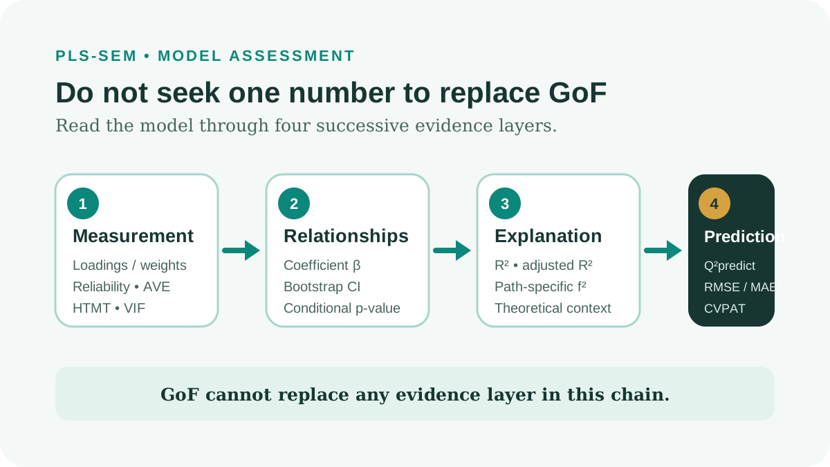
| Assessment layer | Question | Main output |
|---|---|---|
| Measurement model | Do indicators measure the intended constructs? | Outer loadings or weights, reliability, AVE, HTMT, VIF |
| Structural relationships | What are the direction and uncertainty of relationships? | β, bootstrap CIs and p-values |
| In-sample explanation | How much variance does the model explain? | R² and adjusted R² |
| Individual contribution | How much does Y’s R² decrease when X is removed? | f² for each path |
| Out-of-sample prediction | How well does the model predict held-out data? | Q²predict, RMSE or MAE, LM benchmark |
| Predictive ability test | Is PLS-SEM error lower than the benchmark? | CVPAT and loss differences |
3. Prerequisites before interpreting R² and prediction
Assess the structural model only after evaluating measurement according to construct type. For reflective measures, examine outer loadings, reliability, convergent validity and discriminant validity. For formative constructs, prioritize outer weights, collinearity and content coverage.
Keep the model specification consistent across the PLS-SEM Algorithm, bootstrapping and PLSpredict. If indicators, observations or paths change between runs, the tables no longer describe the same model. Save data, model and settings versions before comparing results.
- Identify reflective or formative measurement.
- Complete the appropriate reliability and validity assessments.
- Inspect VIF and estimation warnings.
- Keep data, model and settings consistent across procedures.
- State explanatory, predictive or combined objectives in advance.
4. Interpret R², adjusted R² and f² at the correct level
R² is the proportion of each endogenous variable’s variance explained in-sample by its predictors. Adjusted R² accounts for predictor count and sample size. When comparing models with different predictor counts, adjusted R² reduces the tendency to favor a model simply for including more variables.
f² measures the reduction in R² when a predictor is removed: f² = (R² full - R² excluded)/(1 - R² full). Values of 0.02, 0.15 and 0.35 are commonly used anchors for small, medium and large effects (Cohen, 1988). These are guidelines; practical meaning depends on the field, measurement reliability and research question.
Path coefficients, confidence intervals and f² are not interchangeable. A small p-value with very low f² may indicate a statistically stable but small explanatory contribution. A relatively large f² with a wide CI also requires caution.
| Excluded predictor | Full-model R² | R² after exclusion | f² | Interpretation |
|---|---|---|---|---|
| Trust | 0,520 | 0,470 | 0,104 | Small contribution under Cohen’s anchors |
| Service quality | 0,520 | 0,505 | 0,031 | Small contribution |
| Perceived price | 0,520 | 0,519 | 0,002 | Very small contribution in this model |
For Trust, f² = (0.520 - 0.470)/(1 - 0.520) = 0.104. This constructed example illustrates the formula and is not a result from an empirical study.
5. Distinguish blindfolding Q² from Q²predict
Stone–Geisser Q² from blindfolding assesses predictive relevance by omitting and reconstructing points within the existing sample. It is not out-of-sample prediction in the sense of training on one portion and predicting a held-out portion.
SmartPLS 4 discontinued blindfolding and recommends PLSpredict and CVPAT for out-of-sample predictive assessment (SmartPLS, n.d.-b). Do not search for a Blindfolding button in SmartPLS 4 or relabel Q² from older materials as evidence of prediction on new data.
Positive Q²predict means PLS-SEM error is lower than the mean-prediction benchmark for that indicator. This alone is insufficient: also compare PLS-SEM RMSE or MAE with the linear-model benchmark for each endogenous indicator (Shmueli et al., 2019; SmartPLS, n.d.-c).
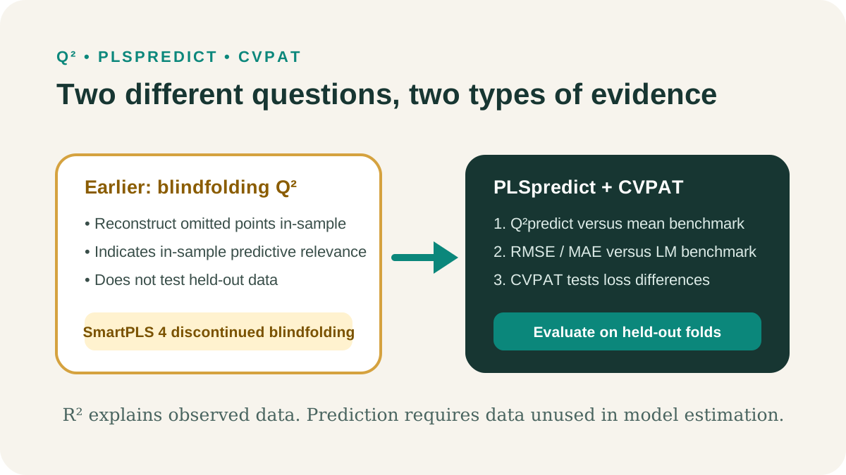
| Result | Evaluation data | Question answered |
|---|---|---|
| Q² blindfolding | Reuses the existing sample | Does the model show in-sample predictive relevance? |
| Q²predict | Held-out folds | Does PLS-SEM outperform the mean benchmark? |
| RMSE or MAE versus LM | Held-out folds | Does the theoretical model outperform the linear benchmark? |
| CVPAT | Cross-validated errors | Does the loss difference support better prediction than the benchmark? |
6. What does CVPAT add to PLSpredict?
PLSpredict supplies prediction errors for descriptive comparisons. CVPAT tests cross-validated loss differences between PLS-SEM and a benchmark. It was developed to compare models or benchmarks on held-out data (Liengaard et al., 2021).
A favorable SmartPLS conclusion requires lower PLS-SEM loss. If the difference is PLS loss minus benchmark loss, only a negative value indicates lower error. Check the direction displayed in your version rather than relying on the p-value alone.
A small p-value does not establish practical importance. Report the benchmark, loss function, folds, repetitions, loss difference and test result. SmartPLS currently includes CVPAT in the PLSpredict report (SmartPLS, n.d.-d).
7. Practical workflow in SmartPLS 4
Menu names may vary slightly between releases. The workflow focuses on assessment logic. Record the SmartPLS version, random seed and cross-validation settings for reproducibility.
Run the PLS-SEM Algorithm
From Calculate, select PLS-SEM Algorithm. Under Quality criteria, record R-square and R-square adjusted for every endogenous variable.
Read f-square
Open the f-square table. Match predictor rows to endogenous-variable columns; do not confuse f² with path coefficients.
Run bootstrapping
Report paths, CIs and p-values. Combine them with f² to distinguish uncertainty from explanatory contribution.
Run PLSpredict/CVPAT
From Calculate, choose PLSpredict/CVPAT. Record folds, repetitions and random seed. SmartPLS describes ten folds and ten repetitions as defaults, but each fold must contain enough observations for estimation.
Read Q²predict
Inspect each endogenous indicator. Positive Q²predict means PLS-SEM outperforms the mean benchmark for that indicator.
Compare RMSE or MAE
Justify the error measure and compare PLS-SEM with LM for each indicator. Do not select the measure after inspecting results to obtain a favorable conclusion.
Read CVPAT
Identify the benchmark and loss-difference direction. Conclude better performance only when PLS-SEM loss is lower and the test supports that difference.
Colors are visual aids. Scientific reporting needs values, benchmarks, settings, criterion sources and limits on the conclusion.
8. Hypothetical example: explanation and out-of-sample prediction
Suppose Loyalty is predicted by Satisfaction, Trust and Switching Costs. Loyalty has R² = 0.610 and adjusted R² = 0.602. Removing Trust reduces R² to 0.550, giving Trust f² = (0.610 - 0.550)/(1 - 0.610) = 0.154.
For LOY1, Q²predict = 0.180. PLS-SEM RMSE is 0.720, below LM RMSE of 0.760. This favors LOY1 predictions against the two benchmarks examined. It cannot be generalized to the entire Loyalty construct before checking the remaining indicators.
Suppose CVPAT yields PLS-minus-LM loss = -0.014 with p = 0.031. Once that difference direction is confirmed, the result supports lower PLS-SEM loss than LM. All numbers in this section are hypothetical illustrations.
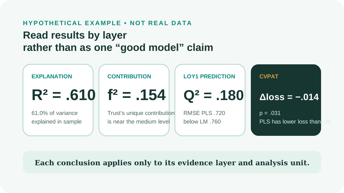
| Layer | Result | Limited conclusion |
|---|---|---|
| Explanation | R² = 0.610; adjusted R² = 0.602 | The model explains 61.0% of in-sample variance |
| Contribution | Trust f² = 0.154 | Contribution near Cohen’s medium anchor |
| Mean benchmark | Q²predict LOY1 = 0.180 | PLS-SEM outperforms the mean benchmark for LOY1 |
| Benchmark LM | RMSE PLS = 0.720; RMSE LM = 0.760 | PLS-SEM has lower error for LOY1 |
| CVPAT | Loss difference = -0,014; p = 0,031 | Evidence of lower PLS than LM loss under the stated direction |
9. Common interpretation errors
| Weak statement | Problem | Correction |
|---|---|---|
| High GoF establishes fit | GoF does not consistently diagnose misspecification | Do not use GoF to accept the model |
| High R² establishes strong prediction | R² is an in-sample result | Run PLSpredict and CVPAT |
| Positive Q² establishes strong prediction | May refer to blindfolding or only a mean-benchmark comparison | Specify Q²predict and compare RMSE/MAE with LM |
| p < 0.05 means a large effect | Statistical significance is not effect magnitude | Report β, CIs and f² |
| Significant CVPAT means a good model | Loss-difference direction has not been checked | Confirm lower PLS than benchmark loss |
| One well-predicted indicator validates the whole scale | The conclusion exceeds the unit evaluated | Inspect every endogenous indicator |
10. APA 7 reporting template and checklist
The template uses the hypothetical example’s numbers. Replace them with actual results and maintain consistent decimal precision.
Reporting example in English
GoF was not used as an overall fit criterion because it does not reliably distinguish correct from misspecified models. The model explained 61.0% of Loyalty variance (R² = .610; adjusted R² = .602). Trust had β = [ ], bootstrap 95% CI [ ; ], p = [ ], and f² = .154. PLSpredict used [k] folds, [r] repetitions and random seed [ ]. For LOY1, Q²predict = .180; PLS-SEM RMSE (.720) was lower than LM (.760). CVPAT indicated PLS-minus-LM loss of -.014, p = .031, supporting lower PLS-SEM loss under the stated benchmark and loss function.
- Do not use GoF to establish fit.
- Report R² and adjusted R² for each endogenous variable.
- Match f² to the correct path and interpret it with β and its CI.
- Distinguish blindfolding Q² from Q²predict.
- State folds, repetitions, random seed and error measure.
- Compare each indicator with the mean and LM benchmarks.
- Read the CVPAT loss-difference direction correctly.
- Separate in-sample explanation from out-of-sample prediction.
Conclusion
GoF is part of the history of PLS path modeling, but should not certify model fit. Updating practice involves more than deleting one statistic from a table.
A current report needs a chain of evidence: measurement quality, coefficients and CIs, R², f², PLSpredict and CVPAT. This requires answering the relevant questions rather than searching for a single number.
References
- Cohen, J. (1988). Statistical power analysis for the behavioral sciences (2nd ed.). Lawrence Erlbaum Associates.https://doi.org/10.4324/9780203771587
- Henseler, J., & Sarstedt, M. (2013). Goodness-of-fit indices for partial least squares path modeling. Computational Statistics, 28(2), 565-580.https://doi.org/10.1007/s00180-012-0317-1
- Liengaard, B. D., Sharma, P. N., Hult, G. T. M., Jensen, M. B., Sarstedt, M., Hair, J. F., & Ringle, C. M. (2021). Prediction: Coveted, yet forsaken? Introducing a cross-validated predictive ability test in partial least squares path modeling. Decision Sciences, 52(2), 362-392.https://doi.org/10.1111/deci.12445
- Shmueli, G., Sarstedt, M., Hair, J. F., Cheah, J.-H., Ting, H., Vaithilingam, S., & Ringle, C. M. (2019). Predictive model assessment in PLS-SEM: Guidelines for using PLSpredict. European Journal of Marketing, 53(11), 2322-2347.https://doi.org/10.1108/EJM-02-2019-0189
- SmartPLS. (n.d.-a). Goodness of fit (GoF) index in PLS-SEM: Why it is limited.https://smartpls.com/documentation/algorithms-and-techniques/validity-and-model-fit/goodness-of-fit/
- SmartPLS. (n.d.-b). Blindfolding and Stone-Geisser's Q² in PLS-SEM.https://smartpls.com/documentation/algorithms-and-techniques/resampling-and-inference/blindfolding/
- SmartPLS. (n.d.-c). PLSpredict: Assessing predictive power in PLS-SEM.https://smartpls.com/documentation/algorithms-and-techniques/prediction-and-segmentation/predict/
- SmartPLS. (n.d.-d). Cross-validated predictive ability test (CVPAT) in PLS-SEM.https://smartpls.com/documentation/algorithms-and-techniques/resampling-and-inference/cvpat/
- Tenenhaus, M., Esposito Vinzi, V., Chatelin, Y.-M., & Lauro, C. (2005). PLS path modeling. Computational Statistics & Data Analysis, 48(1), 159-205.https://doi.org/10.1016/j.csda.2004.03.005
Methodological note: Example values are hypothetical. Interface and command descriptions refer to SmartPLS 4; record the version and consult official documentation if menus change.