
Interpreting Moderation with Graphs: Simple Slopes, Johnson–Neyman, and Confidence Intervals
A plot does not establish moderation. It interprets an estimated interaction coefficient alongside simple slopes, confidence intervals and the observed data range.
A sound workflow retains main effects, tests X × M first, selects meaningful moderator values, calculates predictions from the same equation and interprets simple slopes or Johnson-Neyman regions only within supported data ranges.
Moderation changes the slope of X → Y
- Predictor X
The focal relationship
- Outcome Y
The outcome being explained
- Moderator W
The context of the X → Y relationship
Conceptual diagram. Read the interaction alongside conditional slopes and confidence intervals.
Source: Lê Minh · Conceptual illustration, not software output.1. Learning objectives and prerequisites
This guide teaches you to interpret interaction coefficients, calculate X's conditional effect on Y, select M values for plotting, tabulate predictions, read simple slopes and determine when Johnson-Neyman regions are meaningful.
The model must include X, M and X × M, estimated using disclosed coding and scales. Without the interaction coefficient, standard errors or coefficient covariance matrix, plots remain descriptive illustrations and cannot support inference (Aiken & West, 1991; Hayes, 2022).
- The model includes X, M and X × M.
- Main effects are retained.
- Coding and the 0 points of X and M are stated.
- Data support the intended plotted M values.
- Coefficients and SEs or covariances needed for CIs are available.
- Covariates are held fixed under a disclosed rule.
2. From the interaction equation to conditional effects
For the linear model Y = b0 + b1X + b2M + b3XM, X's conditional effect on Y at M = m is b1 + b3m. Coefficient b3 tests whether X's slope changes with M. Its sign therefore indicates the direction of slope change, rather than establishing X's significance at every M value (Hayes, 2022).
Main effect b1 is X's effect when M equals 0. Main effect b2 is M's effect when X equals 0. If 0 is out of range or lacks meaning, main effects are difficult to interpret even when the interaction is correctly estimated.
Brambor, Clark and Golder (2006) emphasize retaining relevant lower-order terms in interaction models. Removing X or M because of large p-values changes model restrictions and often complicates b3's interpretation.
Every plotted line must come from the same estimated model. Do not draw separate group trend lines and call this moderation without testing the interaction coefficient.
3. Centering, scaling and the meaning of 0
Mean-centering M moves 0 to the sample mean and makes b1 easier to interpret. Centering does not remove interactions or change b3 or fitted values in the same linear model when all components are transformed consistently (Aiken & West, 1991).
Centering can reduce nonessential multicollinearity between products and their components, but does not correct poor measurement or restricted M ranges. Standardizing changes coefficient units, so state whether plots use original, z-standardized or centered scores.
For binary moderators coded 0 and 1, b1 is X's slope in reference group M = 0, and b3 is the between-group slope difference. Do not apply mean ± one SD to grouping variables.
| Form of M | 0 point | b1 | Plotting approach |
|---|---|---|---|
| Continuous, original scale | Actual value 0 | X's slope at M = 0 | Meaningful in-range values |
| Continuous, mean-centered | Sample mean | X's slope at mean M | Percentiles or supported mean ± SD values |
| Continuous, z-score | Sample mean | Slope on the one-SD scale of M | M = -1, 0, 1 if supported by data |
| Binary 0/1 | Reference group | Group 0 slope | One line per group |
| Nominal, K groups | Reference group | Reference-group slope | K lines from K - 1 dummies and interactions |
4. Choose moderator levels for plotting
Mean ± one SD is a convention rather than a requirement. For highly skewed or bounded M, these points may be rare or outside the data. Alternatives include percentiles 16, 50 and 84, substantively meaningful benchmarks or actual group values.
Each plotted level needs an observation count or at least a statement of support. Avoid extending lines into X–M combinations that scarcely occur together. Unsupported extrapolation can look attractive without data evidence.
For few-category ordinal M, plot observed or meaningful categories instead of assuming equal spacing without explanation. If continuous M is grouped only for illustration, retain it as continuous in the primary test unless the hypothesis actually concerns categories.
| Situation | Values to consider | Required checks |
|---|---|---|
| Approximately symmetric distribution | Mean, mean ± 1 SD | All three points are in range |
| Skewed distribution | Percentiles 16, 50, 84 | Observation counts near each point |
| Substantive thresholds exist | Meaningful low, standard and high benchmarks | Thresholds were prespecified |
| Binary moderator | 0 and 1 | Reference group and group sizes |
| Multicategory moderator | Each group | Dummy coding and data per group |
5. Calculate predictions with consistent covariate handling
For a line at M = m, substitute m and a sequence of X values into the estimated equation. Covariates must be fixed at disclosed values, or marginal predictions averaged across the sample distribution can be used. These approaches answer different questions and may yield different predicted Y levels.
Use interpretable Y-axis units. In linear regression, predicted Y is on the outcome scale. With nonlinear links, distinguish link-scale predictions from probabilities or response-scale predictions.
Line confidence intervals cannot be calculated from b1's or b3's SE alone. They require all variances and covariances of the linear combination. Use interaction-probing software or code to avoid omitting covariance terms (Bauer & Curran, 2005).
Step 1
Record the equation, coding and unstandardized coefficients from the final model.
Step 2
Select supported M levels and justify them.
Step 3
Select X values within the common observed range across M levels.
Step 4
Fix or average covariates under a disclosed rule.
Step 5
Calculate predicted Y and CIs from the complete coefficient covariance matrix.
Step 6
Plot lines, CI ribbons and clear coding legends.
Step 7
Verify selected plot points through hand calculations.
Step 8
Retain plotting data with code or spreadsheets.
6. What question do simple slopes answer?
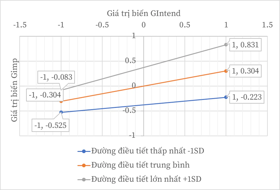
A simple slope is X's effect on Y at a specific M value. Report its estimate, SE or CI and the probed M value. One slope having a small p-value while another has a large one does not establish a difference between slopes. That evidence comes from b3 or a direct contrast.
Bauer and Curran (2005) explain how probing clarifies interaction patterns after testing the product coefficient. Three slopes are only a summary. Nonlinear slope changes or higher-order interactions need appropriate formulas and plots.
With categorical moderators, simple slopes are group-specific slopes. With continuous moderators, each slope is one point on b1 + b3m. Do not describe slopes at mean ± SD as low and high effects for every individual.
Do not conclude moderation because one simple slope has p < 0,05 and another p > 0,05. Directly test the interaction coefficient or slope difference.
7. Johnson-Neyman regions and interpretation limits
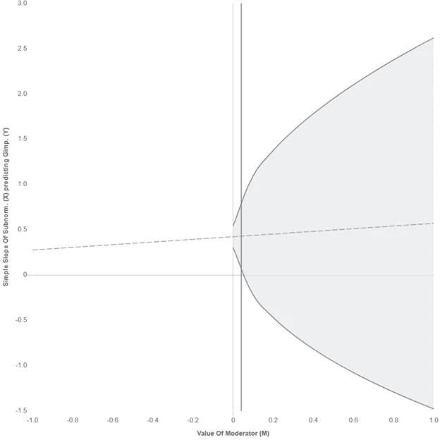
Johnson-Neyman identifies M values where X's conditional effect switches between significant and nonsignificant at the chosen alpha. It uses estimates and coefficient variance-covariance information rather than probing only three points (Bauer & Curran, 2005; Preacher, Curran & Bauer, 2006).
Johnson-Neyman boundaries are not natural thresholds for people or organizations. They depend on sample, model, alpha, estimator and standard errors. Do not turn a value such as 3,42 into an exact policy threshold without supporting data and measurement precision.
Interpret only regions with sufficient observed M values. If the boundary lies outside support, the practical conclusion is that significance status does not change within the observed range. Johnson-Neyman is inappropriate for categorical moderators.
| Tool | Output | Strength | Limitation |
|---|---|---|---|
| Simple slopes | Effects at selected M values | Easy to interpret and report | Depends on selected points |
| Johnson-Neyman | M regions by inferential status | Uses the full continuum | Can suggest false precision |
| Prediction plot | Y levels across X and M | Shows the pattern | Does not replace testing |
| Slope contrast | Difference between two slopes | Directly tests group questions | Requires correct coding and covariance |
8. Hypothetical numerical example: coefficients to three prediction lines
These simulated values illustrate the calculation. The mean-centered model is Y = 10,00 + 0,40X + 0,25M + 0,20XM. Interaction b3 = 0,20, SE = 0,06, 95% CI [0,08; 0,32]. Each one-unit increase in M raises X's slope by 0,20.
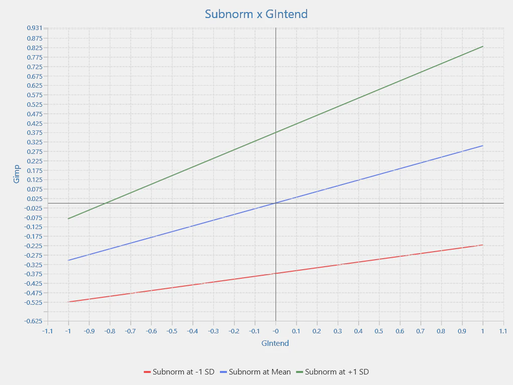
At M = -1, the simple slope is 0,40 + 0,20(-1) = 0,20. At M = 0, it is 0,40. At M = 1, it is 0,60. Suppose probing software gives SEs of 0,08; 0,07 and 0,09; corresponding 95% CIs are [0,04; 0,36], [0,26; 0,54] and [0,42; 0,78].
All three example slopes are positive but increase with M. Plot the common observed X range at the three M levels with CI ribbons. Do not infer that all high-M individuals have higher Y: moderation concerns conditional slopes, not only mean levels.
| M | Formula | X-to-Y slope | Hypothetical SE | Hypothetical 95% CI |
|---|---|---|---|---|
| -1 | 0,40 - 0,20 | 0,20 | 0,08 | [0,04; 0,36] |
| 0 | 0,40 | 0,40 | 0,07 | [0,26; 0,54] |
| 1 | 0,40 + 0,20 | 0,60 | 0,09 | [0,42; 0,78] |
9. Designing an auditable plot
Label axes with variable names, units and ranges. Legends must identify each M level and the selection rule. Use contrasting colors plus line styles so plots remain readable in black and white.
Specify whether ribbons or error bars represent CIs for predicted means or prediction intervals for new observations. These differ. CIs for predicted means or conditional effects often better match moderation inference.
Do not truncate Y merely to exaggerate line differences. If truncation improves detail, disclose it and consider an additional full-range plot. Raw data or partial residuals can be added when sensitive information remains protected.
- X and Y axes include units.
- M levels and coding are explicit.
- The X range remains within support.
- CIs are shown and their type is labeled.
- Colors and line styles are distinguishable.
- Visual intersections are not treated as tests.
- Plotting data are retained.
- Plot values match the simple-slopes table.
10. Common interpretation and presentation mistakes
| Weak practice | Problem | Response |
|---|---|---|
| Two crossing lines establish moderation | Visual crossing is not a statistical test | Report b3 and its CI |
| One slope significant, the other nonsignificant | Does not test their difference | Use the interaction or a contrast |
| Always use mean ± 1 SD | May fall outside support or lack interpretability | Choose justified M values |
| Remove main effects with large p-values | Imposes inappropriate model restrictions | Retain lower-order terms |
| Dichotomize continuous M into high and low | Loses information and power | Keep M continuous for the main test |
| Extend lines beyond the observed range | Unsupported extrapolation | Restrict X and M ranges |
| Omit plot CIs | Conceals uncertainty | Add ribbons or report a CI table |
| Treat J-N boundaries as real cutoffs | Creates false precision | Report uncertainty and support |
11. APA 7 reporting template and completion checklist
The template uses hypothetical values from Section 8. Replace every coefficient, M level and covariate rule with actual results.
Example reporting paragraph
The model included mean-centered X and M and their product X × M. The unstandardized interaction was b = .20, SE = .06, 95% CI [.08, .32], indicating that X's slope increased with M. X's simple slopes at M = -1, 0 and 1 were b = .20, 95% CI [.04, .36]; b = .40, 95% CI [.26, .54]; and b = .60, 95% CI [.42, .78], respectively. The plot shows predicted Y over the common observed X range at these M levels; covariates were held at [rule]. Johnson-Neyman analysis [was/was not] used because of [reason and support].
- Report the interaction coefficient, SE and CI.
- Retain X and M in the model.
- Describe centering or standardization.
- Explain the 0 points of X and M.
- Moderator levels lie within the data.
- Report simple-slope estimates and CIs.
- Do not infer differences from separate p-values.
- Use Johnson-Neyman only for suitable continuous M.
- Limit J-N boundaries to supported ranges.
- Apply clear covariate rules.
- Show CIs and axis units.
- Retain data and plotting code for reproduction.
Conclusion
A good moderation plot visualizes the interaction model rather than providing independent evidence. X × M tests whether slopes change; simple slopes and Johnson-Neyman explain where changes occur.
Trustworthy presentation preserves coding, avoids extrapolation, discloses uncertainty and distinguishes statistical boundaries from practically meaningful thresholds.
References
- Aiken, L. S., & West, S. G. (1991). Multiple regression: Testing and interpreting interactions. SAGE Publications.https://us.sagepub.com/en-us/nam/multiple-regression/book3045
- Bauer, D. J., & Curran, P. J. (2005). Probing interactions in fixed and multilevel regression: Inferential and graphical techniques. Multivariate Behavioral Research, 40(3), 373-400.https://doi.org/10.1207/s15327906mbr4003_5
- Brambor, T., Clark, W. R., & Golder, M. (2006). Understanding interaction models: Improving empirical analyses. Political Analysis, 14(1), 63-82.https://doi.org/10.1093/pan/mpi014
- Hayes, A. F. (2022). Introduction to mediation, moderation, and conditional process analysis: A regression-based approach (3rd ed.). Guilford Press.https://www.guilford.com/books/Introduction-to-Mediation-Moderation-and-Conditional-Process-Analysis/Andrew-Hayes/9781462549030
- Preacher, K. J., Curran, P. J., & Bauer, D. J. (2006). Computational tools for probing interactions in multiple linear regression, multilevel modeling, and latent curve analysis. Journal of Educational and Behavioral Statistics, 31(4), 437-448.https://doi.org/10.3102/10769986031004437
Academic note: Example values were constructed to illustrate calculations. Plots and Johnson-Neyman regions cannot correct misspecification, endogeneity, measurement error or observations outside supported ranges.