
SmartPLS 4 Supports Linear and Logistic Regression alongside PLS-SEM
Most SmartPLS users associate the software with PLS-SEM. A recent Journal of Marketing Analytics tutorial shows its separate multiple linear and logistic regression module, including assumptions, model fit and residual diagnostics within the interface rather than requiring a switch to SPSS or Stata.
Start reading1. SmartPLS extends beyond PLS-SEM
SmartPLS is best known as dedicated PLS-SEM software (Ringle et al., 2024). Margalina et al. (2026), however, describe version 4's expansion into necessary condition analysis (NCA), importance-performance map analysis (IPMA), covariance-based SEM (CB-SEM), generalized structured component analysis (GSCA), and a separate module for multiple linear and logistic regression.
The tutorial motivates this module by observing that familiar statistical interfaces such as SPSS and Stata have changed little over 30 years, often requiring users to move between windows or write syntax to obtain a complete regression output (Margalina et al., 2026). SmartPLS brings the workflow together in one graphical interface, producing tables and charts after estimation.
Many questions do not require a full structural model. Questions about whether X predicts Y or how two customer groups differ may call for linear or logistic regression. A dedicated module allows users familiar with SmartPLS to perform an additional analysis without opening SPSS.
2. Continuous and binary outcomes are different problems
Multiple linear regression explains an interval- or ratio-scaled outcome using several predictors. Logistic regression addresses a binary outcome with two possible values (Margalina et al., 2026). This distinction shapes estimation, assumptions and coefficient interpretation.
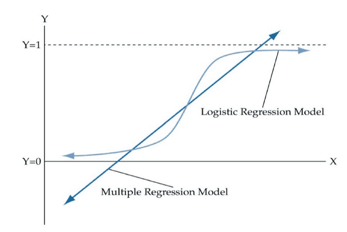
The tutorial illustrates both models using HBAT, a simulated market-segmentation data set for a paper manufacturer used in Multivariate Data Analysis (Hair et al., 2019). Thirteen predictors measure customers' perceptions of HBAT performance (X6 to X18, on a 0–10 scale). The two models use this pool of predictors but different outcomes.
| Model | Outcome | Data type | Predictors |
|---|---|---|---|
| Multiple linear regression | X19, customer satisfaction | Interval, 0–10 scale | HBAT perceptions: X6, X7, X9, X11 and X12, selected theoretically |
| Logistic regression | X4, customer region | Binary: 0 = North America, 1 = outside North America | HBAT perceptions: all X6 to X18 |
Source: Margalina et al. (2026), using Hair et al.'s HBAT data (2019, Chapters 5 and 8).
Margalina et al. (2026) note declining reliance on stepwise, backward and forward selection because these algorithms are not theory-driven and overlook concerns such as collinearity, outliers and influential observations. Because dropping a theoretically important predictor may be riskier than retaining a less relevant one, they favor theoretical model justification over automatic selection.
3. Six stages of regression analysis
Hair et al. (2019) describe six stages for both linear and logistic regression, used as the framework of Margalina et al.'s (2026) tutorial.
Stage 1: Define the objectives
Choose outcomes and predictors and select linear or logistic regression according to the explanatory, predictive or combined objective.
Stage 2: Design the study
Consider sample size and measurement. The tutorial discusses larger sample requirements for logistic regression, estimated by maximum likelihood (ML), compared with OLS linear regression.
Stage 3: Assess assumptions
The assumptions differ; Section 4 explains them.
Stage 4: Estimate and assess overall fit
Estimate the model and inspect overall fit, such as R² for linear regression or likelihood and pseudo R² for logistic regression.
Stage 5: Interpret the variables
Examine each predictor's role through coefficient direction and magnitude.
Stage 6: Assess generalizability
Examine whether performance extends beyond the present sample to the intended population.
4. Why the models require different assumptions
Researchers familiar with linear regression may overlook that its assumptions and diagnostics do not all transfer to logistic regression. Some familiar measures have no direct logistic counterpart.
| Aspect | Linear regression (OLS) | Logistic regression (ML) |
|---|---|---|
| Assumptions | Linearity, random sampling, no perfect multicollinearity, zero conditional error expectation and constant error variance under the Gauss–Markov framework | No perfect multicollinearity, independent observations and a linear relationship between continuous predictors and log-odds, rather than probability |
| Normality, homoscedasticity | Applicable | Not applicable |
| Model fit | R², adjusted R² and ANOVA | Log-likelihood, deviance difference, AIC, BIC, McFadden R², Cox and Snell R², and Nagelkerke R² |
| Statistical significance | t-test | Wald test |
| Coefficient interpretation | Unstandardized and standardized coefficients | Log-odds coefficients and exponentiated coefficients, or odds ratios |
| Interpreting individual predictors | Standardized coefficients | Log-odds coefficients/odds ratios; a confusion matrix assesses whole-model classification, not individual predictor importance |
Source: summarized from Table 3 of Margalina et al. (2026).
Normality and homoscedasticity are not logistic-regression assumptions, so standard linear-model QQ plots or Breusch–Pagan tests do not test required logistic assumptions (Hosmer et al., 2013; Margalina et al., 2026). Relevant checks concern collinearity, observation independence and linearity between predictors and log-odds, not outcome probability.
5. Case 1: multiple linear regression of customer satisfaction
The first model predicts customer satisfaction, X19, using five theoretically selected predictors: product quality (X6), e-commerce activity (X7), complaint resolution (X9), product line (X11) and salesforce image (X12). Its observation-to-predictor ratio is 20:1, meeting the reference level discussed by Hair et al. (2019).
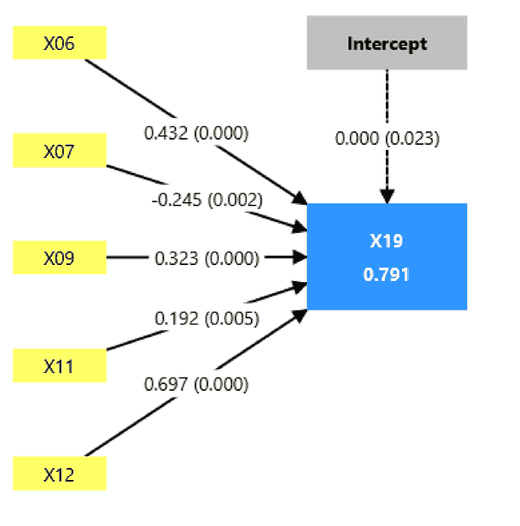
The model F statistic is 71.058 (p < 0.001), with regression sum of squares 111.205 out of total 140.628 (Margalina et al., 2026). Adjusted R² is 0.780, close to the original R² of 0.791; these describe in-sample fit and do not independently establish out-of-sample generalizability. Durbin–Watson is 2.449; proximity to 2 alone does not establish absence of autocorrelation. Interpretation requires the observation order, applicable conditions and an appropriate test result.
| Variable | Unstandardized coefficient | Standardized coefficient (β) | t | p |
|---|---|---|---|---|
| X06, product quality | 0,369 | 0,432 | 7,820 | < 0,001 |
| X07, E-commerce | -0,417 | -0,245 | -3,162 | 0,002 |
| X09, complaint resolution | 0,319 | 0,323 | 5,256 | < 0,001 |
| X11, product line | 0,174 | 0,192 | 2,860 | 0,005 |
| X12, salesforce image | 0,775 | 0,697 | 8,711 | < 0,001 |
| Intercept | -1,151 | 0,000 | 2,303 | 0,023 |
Source: Margalina et al. (2026, Figure 9).
All five coefficients are significant at 0.05 and exceed the 0.10 standardized-coefficient relevance reference used in the tutorial. Salesforce image is the strongest predictor (X12, β = 0.697), followed by product quality (X06, β = 0.432) and complaint resolution (X09, β = 0.323). E-commerce activity (X07) has a negative coefficient: more favorable e-commerce perceptions are associated with lower satisfaction. Margalina et al. (2026) note this counterintuitive finding and refer to Hair et al. (2019, pp. 348–349) for discussion.
The intercept is -1.151 and statistically significant (p = 0.023). It is the prediction when every predictor equals 0; its negative value on the 0–10 scale must be considered alongside data support and the meaning of zero (Margalina et al., 2026). A negative intercept neither implies that Y must equal 0 when all X equal 0 nor independently justifies omitting the intercept. A through-origin model requires theoretical or design support for that restriction; the tutorial retains the intercept.
6. Case 2: logistic regression of customer region
The second model predicts customer region, X4, coded 0 = North America and 1 = outside North America, using all 13 HBAT-perception variables, X6–X18. It uses 100 observations. The 400-observation figure discussed by Margalina et al. (2026) is a tutorial reference benchmark, not a universal maximum-likelihood requirement. Justify sample size using model complexity, event and nonevent counts, intended precision and expected performance rather than one fixed threshold for every logistic regression.
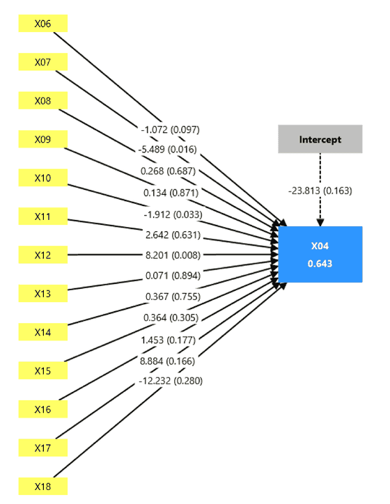
The null model's -2LL is 133.750, decreasing to 30.789 in the estimated model, a substantial improvement over a model without predictors (Margalina et al., 2026). All three pseudo R² values exceed 0.5: McFadden 0.770, Cox and Snell 0.643 and Nagelkerke 0.872.
| Variable | Coefficient (log-odds) | Wald | p | Odds ratio Exp(B) |
|---|---|---|---|---|
| X07, E-commerce | -5,489 | 5,851 | 0,016 | 0,004 |
| X10, advertising | -1,912 | 4,537 | 0,033 | 0,148 |
| X12, salesforce image | 8,201 | 6,957 | 0,008 | 3.645,181 |
Only the 3 predictors significant at 0.05 are listed out of 13. Source: Margalina et al. (2026, Figure 22).
E-commerce (X07) and advertising (X10) have negative coefficients: higher perceptions of these factors are associated with lower odds of belonging to the outside-North-America group. Salesforce image (X12) has a large positive coefficient, indicating higher odds of that group as its rating increases.
X12's coefficient, 8.201, has a relatively large standard error, 3.109, producing an odds ratio above 3,600. An unusually large logistic coefficient and standard error in a binary-outcome sample of only 100 can indicate quasi-complete separation, rather than an exceptionally strong causal relationship. Examine the predictor's distribution in both groups before interpreting such values.
7. Interpreting logistic coefficients: log-odds, Wald and odds ratios
Logistic regression models the natural logarithm of the odds, the ratio of outcome occurrence to nonoccurrence probability, as a linear function of predictors (Margalina et al., 2026).
The sigmoid function converts log-odds to probability:
A β coefficient represents log-odds rather than probability, so it cannot be read like a linear-regression coefficient. Exponentiating it gives the odds ratio Exp(B): above 1 indicates a positive association, below 1 a negative association, and 1 no association (Margalina et al., 2026).
Do not report raw logistic β as a probability change. Obtain Exp(B), then calculate the percentage change in odds as [Exp(B) - 1] × 100%. For X07, Exp(B) = 0.004, so odds decrease by 99.6% per 1-point increase in e-commerce perceptions; for X10, Exp(B) = 0.148, odds decrease by 85.2%.
Sample logistic-regression interpretation
The logistic coefficient for [variable] was [β] (Wald = [value], p = [value]), corresponding to Exp(B) = [value]. A 1-unit increase in [variable] was associated with a [percentage]% [increase/decrease] in the odds of [outcome = group 1], holding the other predictors constant.
| Incorrect wording | Why it is incorrect | Better wording |
|---|---|---|
| β = 8.201 means that a 1-point increase in X12 increases probability 8.201 times | β is log-odds, not probability or an odds ratio | Exponentiate β to obtain Exp(B) = 3,645.181, then interpret the odds ratio |
| Nagelkerke R² = 0.872 means 87.2% of variance is explained | This is pseudo R², not the proportion of variance explained in the OLS sense | Nagelkerke R² = 0.872 describes fit relative to the null model, not a percentage of variance explained |
| Using QQ plots or Breusch–Pagan to test logistic assumptions | Normality and homoscedasticity are not logistic-regression assumptions | Check collinearity, independence and linearity between continuous predictors and log-odds |
8. Limitations reported for the SmartPLS regression module
Margalina et al. (2026) describe logistic regression in SmartPLS as beta at the time of their tutorial. They identify two missing diagnostics relative to SPSS or Stata: ROC curves for predictive discrimination and Box–Tidwell assessment of linearity between predictors and log-odds. They also report Box–Tidwell as unavailable in the linear-regression module.
- The model type, linear or logistic, fits the outcome's measurement level.
- Predictors were selected through theoretical justification rather than automatic selection.
- Collinearity was checked using VIF and condition indices in both model types.
- For linear regression, residual patterns, Breusch–Pagan, Durbin–Watson and QQ plots were examined.
- For logistic regression, normality/homoscedasticity tests were not imposed, and coefficients were interpreted through Exp(B) rather than raw β.
- Sample size was considered for the particular model, especially logistic regression.
- Unusual coefficients and standard errors were checked for possible quasi-complete separation in small samples.
Conclusion
Adding linear and logistic regression expands what familiar SmartPLS users can do in one interface without replacing SPSS or Stata for every regression task. The priority is understanding the different questions, assumptions, fit measures and coefficient interpretations. Applying one model's diagnostics mechanically to the other is a common mistake, regardless of software.
References
Primary SmartPLS and regression source
- Margalina, V.-M., Kreienbaum, C., Hair, J. F., Becker, J.-M., & Ringle, C. M. (2026). Multiple linear and logistic regression analysis: a SmartPLS 4 software tutorial. Journal of Marketing Analytics, 14, 709-726. https://doi.org/10.1057/s41270-026-00466-2
- Ringle, C. M., Wende, S., & Becker, J.-M. (2024). SmartPLS 4. Bönningstedt: SmartPLS. https://www.smartpls.com
Foundational regression sources
- Hair, J. F., Black, W. C., Babin, B. J., & Anderson, R. E. (2019). Multivariate data analysis (8th ed.). Cengage Learning.
- Hosmer, D. W., Lemeshow, S., & Sturdivant, R. X. (2013). Applied logistic regression (3rd ed.). Wiley.
Academic note: This article summarizes a published software tutorial and does not replace official SmartPLS documentation. All numerical examples use the HBAT sample data in Margalina et al. (2026) and Hair et al. (2019); users must assess assumptions and sample adequacy for their own models. Figures are reproduced from Margalina et al. (2026), published under Creative Commons Attribution 4.0 International (CC BY 4.0), permitting reproduction and adaptation with attribution.
R Core Team. Summarizing linear model fits.