
PLS-MGA and MICOM: Comparing Groups Without Overlooking Measurement Invariance
Before comparing paths across groups, establish whether the composites are formed comparably. MICOM answers this by step and construct, rather than awarding a green label to the whole model.
Document configuration, compare c with its permutation boundary, then locate mean and log-variance differences within reference intervals. Partial and full invariance have different scope; one composite cannot stand in for every relationship in a model.
Group comparisons start with equivalence
- Define groups
Explicit theory and group coding
- Measurement invariance
Check whether comparisons are valid
- Compare paths
Test the difference directly
- Interpretation
Report sample sizes and limitations
Conceptual diagram. Different p-values do not by themselves establish different coefficients.
Source: Lê Minh · Conceptual illustration, not software output.1. What MICOM makes comparable
Group coefficients may differ because structural relationships differ, or because a scale with the same name forms a different measure in each group. MICOM examines the comparability of composites before interpreting group differences. Henseler, Ringle, and Sarstedt (2016) developed the procedure for composites; the metric and scalar labels of multigroup CFA should not simply be transferred to MICOM.
Failure to reject invariance does not prove that the groups are identical. Sample size, precision and specification still constrain the ability to detect differences. Report evidence supporting invariance under the tested configuration rather than certain equivalence across every population (Henseler et al., 2016; Hair et al., 2018, Chapter 4).
2. Three sequential questions
Hair et al. (2018, Chapter 4) describe MICOM as a conditional sequence: shared configuration first, comparable score composition next, then means and variances. Do not compress the output into one model-wide pass/fail label when composites have different results.
| Step | Evidence to retain | Interpretation |
|---|---|---|
| 1. Configural | Indicators, scales, data treatment, algorithm | Inspect the records; a p-value cannot replace this |
| 2. Compositional | Observed c, permutation quantile and corresponding p | Check whether c lies in the lower reference tail |
| 3. Mean/variance | Observed differences and permutation intervals for each quantity | Locate each observed difference relative to its interval; do not just look for zero |
Steps 1 and 2 support partial invariance. Adding equality of means and variances in Step 3 supports full invariance for the composite assessed. Full invariance does not establish equal path coefficients; MGA must still examine that question (Hair et al., 2018, Chapter 4).
3. Step 1: inspect configuration before estimation
An identical diagram is not sufficient for configural invariance. Hair et al. (2018, Chapter 4) require matching indicators and scales, data-treatment procedures, algorithms and settings. Translated items also need evidence of content equivalence; matching variable names do not establish it.
Keep a configuration record for each group: original and reverse-coded values, missing-data rules, standardization, outlier handling, final items and estimation settings. A common treatment rule does not require identical missingness rates or distributions. If the model changes after inspecting MICOM, rerun the assessment and record the reason (Hair et al., 2018, Chapter 4).
- Matching content domain, indicators and coding direction.
- Matching data-treatment rules and observation-selection criteria.
- Matching model type, algorithm and comparison settings.
- Retain configuration evidence rather than waiting for a Step 1 p-value.
4. Step 2: interpret c against the permutation distribution
Step 2 examines equivalent composite composition; it does not test Cronbach's alpha or HTMT. At alpha = .05 in the procedure described by Hair et al. (2018, Chapter 4), compare observed c with the fifth percentile of the permutation c distribution. An observed value below this boundary does not support compositional invariance; a value above it is not rejected by that test.
Do not round c to 1.000 before deciding. Two values both displayed as .99 can fall on opposite sides of the boundary at higher precision. Near the boundary, inspect output precision, permutation count and sensitivity rather than changing alpha after seeing the result.
For a single-item variable, c = 1 follows from score construction and does not provide the informative compositional test available for a multi-item scale. Inspect the variable definition, coding direction and model role. A c of 1 does not establish the reliability or validity of a single-item measure (Hair et al., 2018, Chapter 4).
5. Step 3: use the correct difference and reference interval
In Step 3, scores used for mean and variance comparisons come from estimation on the pooled data and are then assigned to groups. This is not a comparison of two separately standardized group-score sets, which can remove the very differences of interest (Hair et al., 2018, Chapter 4).
The mean statistic is Δμ = mean_A − mean_B. The variance statistic is log(var_A/var_B), equivalently log(var_A) − log(var_B). Compare each observed difference with its corresponding permutation interval. Hair et al. (2018, Chapter 4) use this interpretation; the SmartPLS MICOM documentation also corrects earlier wording in Henseler et al. (2016) to avoid checking only whether an interval contains zero. See also the current MICOM guidance (SmartPLS, n.d.-a).
Failure at Step 3 does not automatically remove partial invariance supported by Steps 1 and 2. Report means, variances and composition separately for each composite. A variance difference does not establish that a structural path differs between groups.
6. Constructed example: compositional results by construct
The table illustrates interpretation at alpha = .05. Its c values and quantiles are constructed to demonstrate contrasting cases, not estimated from a fitted dataset. Assume Step 1 has been documented. Trust and Quality exceed the fifth-percentile boundary, whereas Intention falls below it despite a correlation close to 1.
| Composite | Observed c | 5% quantile | Interpretation |
|---|---|---|---|
| Trust | 0.998 | 0.992 | Composition not rejected |
| Quality | 0.997 | 0.991 | Composition not rejected |
| Intention | 0.985 | 0.990 | Composition not supported |
| Single-item variable | 1.000 | 1.000 | Not a validation of measurement quality |
Composition is not supported for Intention in this example. Do not interpret MGA paths involving that composite as if comparability had been established. Inspect coding and content; justify any respecification theoretically and rerun MICOM. Do not delete a construct simply to obtain a favorable table (Hair et al., 2018, Chapter 4).
7. Worked continuation: an interval containing zero can still fail Step 3
Continue only with the two composites supported at Step 2. Trust has an observed log-variance difference of .30, outside [−.18, .18]. That interval contains zero but not .30, so equality of variances is not supported. Trust has partial evidence, while Quality also has Step 3 evidence. Intention still failed Step 2 and cannot be ignored in a model-wide statement.
| Composite / quantity | Observed difference | Permutation interval | Observed value inside? |
|---|---|---|---|
| Trust / mean | 0.12 | [−0.20, 0.20] | Yes |
| Trust / log variance | 0.30 | [−0.18, 0.18] | No |
| Quality / mean | −0.08 | [−0.15, 0.16] | Yes |
| Quality / log variance | 0.05 | [−0.17, 0.17] | Yes |
# Constructed summary values, not a MICOM estimation pipeline.
observed <- c(0.12, 0.30, -0.08, 0.05)
lower <- c(-0.20, -0.18, -0.15, -0.17)
upper <- c( 0.20,  0.18,  0.16,  0.17)
inside <- observed >= lower & observed <= upper
data.frame(observed, lower, upper, inside)
# Expected: TRUE FALSE TRUE TRUE
log(1.35 / 1.00) # 0.3001046, approximately 0.30 in the table
stopifnot(identical(inside, c(TRUE, FALSE, TRUE, TRUE)))
8. SmartPLS workflow and records to retain
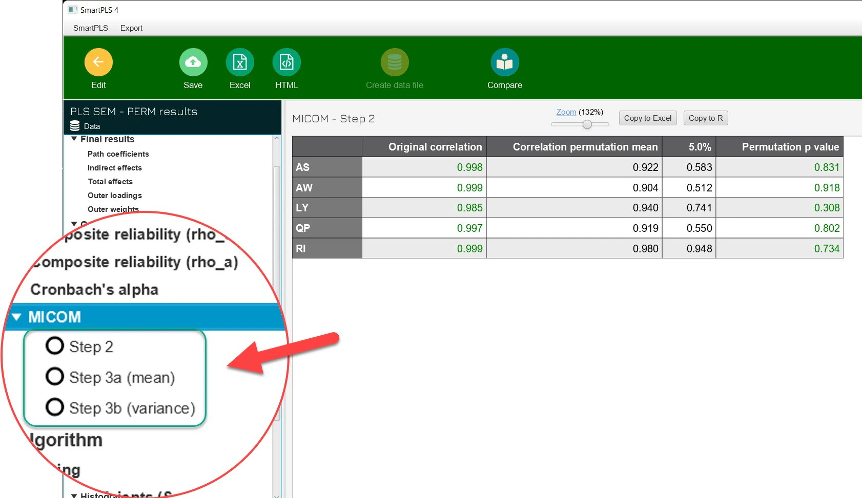
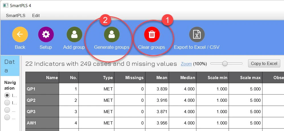
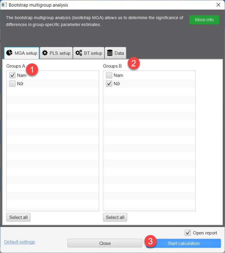
In SmartPLS, create data groups and use Permutation to inspect the MICOM tables. Keep the estimator consistent; do not compare one PLS group with another estimated using PLSc. Record the version, A/B groups, permutation count, alpha and seed where exposed. Match the computation effort to the purpose and revisit results near the boundary (SmartPLS, n.d.-b).
Define groups and the comparison
Record grouping rules, usable group sizes and the paths of interest.
Document configuration
Compare indicators, treatment and settings; retain Step 1 evidence.
Read Step 2 by composite
Retain c, its reference boundary and the decision; flag single-item variables.
Read means and variances
Locate each observed difference within its interval and identify the variance statistic.
Define the scope of MGA
Do not claim model-wide invariance when a relevant composite remains unsupported.
Save results and decisions
Retain unfavorable results, justified changes and rerun records.
9. When invariance is not supported
First inspect checkable causes: incorrect reverse coding, questionnaire versions, different item deletions, missing-data treatment or algorithm settings. Correct genuine errors under a common rule and rerun. If the issue concerns scale content, revisit the theory and instrument rather than only increasing permutation counts (Hair et al., 2018, Chapter 4).
Unsupported invariance does not prove fabricated data or poor responses in one group. Conversely, a null finding in a small group does not prove equivalent measurement. Report group models within a defensible scope, disclose comparison limits and distinguish predefined groups from exploratory FIMIX/PLS-POS segments.
10. Report each composite and each step
Following Henseler et al. (2016) and Hair et al. (2018, Chapter 4), report configuration evidence, composition, then means and variances. State that full invariance does not imply equal paths. For path comparisons, continue to the practical PLS-MGA guide after defining the scope of supported invariance.
Suggested reporting text
MICOM compared [Group A, n] with [Group B, n]. Configural invariance was documented through [indicators, coding, treatment and algorithm]. With [number] permutations and alpha = [ ], compositional invariance was supported for [list] but not for [list]. At Step 3, the observed [mean/log-variance difference] for [composite] lay [inside/outside] the reference interval [ ]. Structural comparisons were therefore restricted to [state scope], rather than claiming invariance for the entire model.
- Retain c and its permutation boundary without premature rounding.
- Distinguish a variance difference from a log-variance difference.
- Compare Step 3 intervals with observed differences, not only zero.
- Identify single-item variables and unsupported composites.
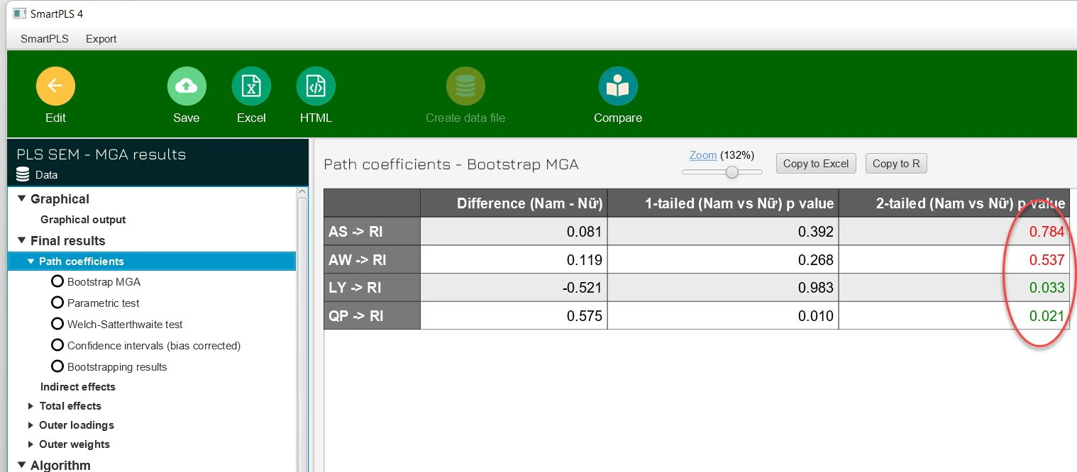
- Keep original screenshot values separate from constructed examples.
Conclusion
MICOM defines the defensible scope of comparison rather than ensuring that every group difference is meaningful. Keep the links between configuration records, c and its reference distribution, means and variances, and each composite.
When Step 2 is unsupported, do not proceed directly to MGA interpretations involving that construct. When only Step 3 is unsupported, state the appropriate limit rather than treating all partial invariance as lost.
References
- Henseler, J., Ringle, C. M., & Sarstedt, M. (2016). Testing measurement invariance of composites using partial least squares. International Marketing Review, 33(3), 405–431. https://doi.org/10.1108/IMR-09-2014-0304
- SmartPLS. (n.d.-a). Measurement invariance assessment (MICOM) in PLS-SEM. https://smartpls.com/documentation/algorithms-and-techniques/heterogeneity-and-multigroup/micom/
- Hair, J. F., Sarstedt, M., Ringle, C. M., & Gudergan, S. P. (2018). Advanced issues in partial least squares structural equation modeling. SAGE. https://us.sagepub.com/en-us/nam/advanced-issues-in-partial-least-squares-structural-equation-modeling/book243803
- SmartPLS. (n.d.-b). Permutation testing for PLS-SEM multigroup analysis. https://smartpls.com/documentation/algorithms-and-techniques/resampling-and-inference/permutation/
Methodological note: Numerical tables are constructed examples for learning to interpret output. The R code checks arithmetic and interval reading; it does not re-estimate MICOM or validate the original screenshot data.