
Analyzing Control Variables in AMOS: Correct Selection, Specification, and Transparent Reporting
Control variables are not a demographic list added to make a model appear rigorous. Each adjusted variable changes the estimand and may reduce or introduce bias.
A sound workflow starts by defining the estimand, drawing assumed causal relationships, selecting the adjustment set before examining p-values, coding variables correctly in AMOS, and comparing unstandardized coefficients and confidence intervals between baseline and adjusted models.
Controls need justification and sensitivity checks
- Theoretical basis
Explain why adjustment is needed
- Coding
Specify type and reference group
- Specification
Include in the relevant equations
- Sensitivity
Compare adjusted and unadjusted results
Conceptual diagram. Adding more controls does not automatically improve inference.
Source: Lê Minh · Conceptual illustration, not software output.1. Learning objectives and prespecified estimands
This guide teaches you to distinguish confounders, mediators and colliders, decide which variables to adjust, enter continuous or categorical variables into AMOS, and assess sensitivity of the main conclusion to the control set.
Define the target quantity before choosing controls. The total effect of X on Y includes valid mediated paths. The direct effect holding a mediator fixed answers a different question. If the target changes across models, a changed X-to-Y coefficient cannot simply be described as better control (Cinelli, Forney & Pearl, 2024).
- Specify X, Y and the target effect.
- Identify when each variable is measured.
- Distinguish total from direct effects.
- Select controls before examining main results.
- Justify each control through theory or design.
- Obtain sufficiently reliable measurements of important controls.
2. Adding a control expresses a causal assumption
In observational data, controls often block back-door paths between X and Y. The simplest case is Z causing both X and Y. Adjusting Z may separate associations outside the causal X-to-Y path, but this depends on the assumed structure rather than correlations or p-values alone (Rohrer, 2018).
Spector and Brannick (2011) caution against automatically adding controls in the hope of purifying relationships. A variable correlated with Y is not necessarily a confounder. A statistically nonsignificant variable may still require adjustment when design and theory indicate that it blocks confounding paths.
AMOS estimates the specified covariance model. Software cannot determine whether a control arrow represents a cause, mediator or collider. Identification of the target quantity remains the responsibility of research design and analytical reasoning.
Do not remove a confounder because p exceeds 0,05 or add a variable simply because it predicts Y. Base decisions on its role in the assumed causal structure.
3. Confounders, mediators, colliders and consequences of X
A confounder is a common cause of X and Y, or a variable helping block an appropriate confounding path. A mediator lies on the X-to-Y path. A collider is a common consequence of two variables. Adjusting a mediator when targeting the total effect blocks part of that effect; adjusting a collider may open a spurious association path (Cinelli et al., 2024).
Variables measured before X are often safer than post-treatment variables, but pre-treatment status does not guarantee a good control. A variable's role also depends on other adjustment-set members. The same Z can help in one structure and introduce bias in another.
State limitations when gender, age or tenure merely proxy the mechanism of interest. Spector and Brannick (2011) recommend avoiding demographic substitutes for the theoretical concepts actually under investigation.
| Assumed role | Example structure | Treatment when estimating total effects | Risk |
|---|---|---|---|
| Confounder | Z causes X and Y | Usually requires adjustment | Omission may introduce confounding |
| Mediator | X causes Z; Z causes Y | Do not adjust when targeting the total effect | Changes total-effect estimation into direct-effect estimation |
| Collider | X causes Z and U causes Z | Do not adjust | Opens spurious association paths |
| Consequence of X | X causes Z | Usually unsuitable as a control | Post-treatment bias |
| Predictor of Y only | Z causes Y but not X | May improve precision when valid | Does not automatically resolve confounding |
4. Choose and measure controls before running AMOS
Becker (2005) and Bernerth and Aguinis (2016) require explanations of considered variables, inclusion/exclusion reasons, measurement and whether conclusions depend on these choices. Saying that prior studies controlled a variable is insufficient when they asked different causal questions.
Poorly measured controls may incompletely block confounding. A single unreliable indicator for an important latent control can leave residual confounding. With multi-item scales and sufficient sample size, a control can be modeled as latent; when using observed totals, disclose scoring and reliability.
Prepare a pre-analysis decision table containing variable names, timing, assumed roles, paths requiring adjustment, coding and sensitivity analyses. This reduces result-driven additions or removals.
| Variable | Assumed role | Timing | Measurement and coding | Decision |
|---|---|---|---|---|
| Age | Confounder under domain theory | Before X | Years, retained as continuous | Include |
| Tenure | Proxy closely related to age | Before X | Years | Check multicollinearity |
| Satisfaction | Hypothesized mediator | After X | 4-item latent variable | Do not control when estimating the total effect |
| Industry group | Background differences | Before X | K groups, create K - 1 dummies | Include if consistent with the DAG |
5. Specifying controls in AMOS
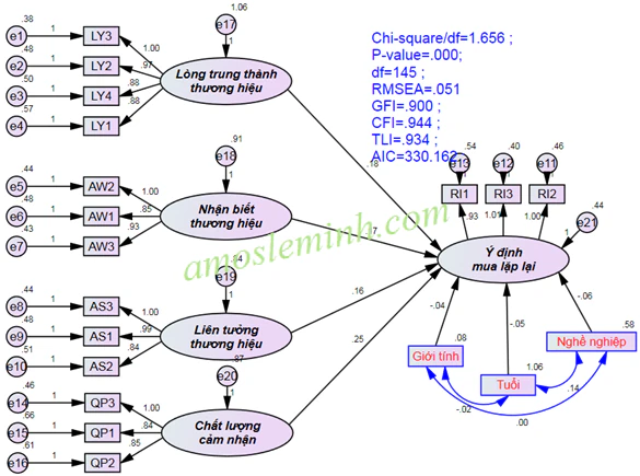
In IBM SPSS Amos 29, an observed control enters as exogenous if it has no explanatory equation in the model. Draw one-headed paths to the specific endogenous variables requiring adjustment. Allow covariances with related exogenous variables when justified by theory. Do not habitually connect controls to every endogenous variable (IBM Corp., 2022).
Latent controls require measurement-model specification and solution checks like other constructs. AMOS does not automatically correct measurement error in observed total scores. These approaches are not equivalent.
Keep the estimator and missing-data treatment consistent between baseline and adjusted models. Different case sets can change coefficients because the sample changed, rather than solely because controls were added.
Step 1
Finalize estimand, adjustment set and baseline model before opening AMOS.
Step 2
Check ranges, missingness, coding and measurement timing for each control.
Step 3
Enter observed or latent controls appropriately and specify reference groups for dummies.
Step 4
Draw control-to-endogenous paths according to the causal graph, rather than p-values.
Step 5
Allow covariance with exogenous predictors when background associations are assumed and need estimation.
Step 6
Estimate baseline and adjusted models using the same dataset.
Step 7
Compare unstandardized coefficients, SEs, CIs, signs and conclusions for the focal path.
Step 8
Retain model files, output and the rationale for every control.
6. Code categorical variables while preserving the research question
A nominal observed predictor with K groups requires K - 1 dummies. The omitted category is the reference group; interpret all coefficients relative to it. Changing the reference group changes coefficient presentation without changing model predictions.
Do not code unordered categories as 1, 2, 3 and treat them as continuous. This imposes unsupported spacing and a linear trend. For ordinal controls, decide between continuous treatment and dummies using category count, relationship shape and objectives.
If the question is whether X-to-Y coefficients differ by group, the grouping variable acts as a moderator. Multigroup SEM and measurement invariance are then often more suitable than calling the group a control.
Controls adjust mean levels or background relationships under a specification. Moderators ask whether X's effect on Y changes with Z. A variable can serve both roles, but models and interpretations must distinguish them.
7. Compare baseline and adjusted models
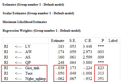
Look beyond control p-values. The key evidence is how the focal coefficient changes under a justified adjustment set. Prioritize unstandardized coefficients and CIs because standardized coefficients can shift as variance is redistributed across models.
Better fit does not establish correct control selection. Adding paths usually lowers sample chi-square. Kline (2023) emphasizes reading fit alongside specification, parameters and inferential objectives. Unjustified controls can still improve fit.
Highly correlated controls can increase standard errors and destabilize coefficient signs. Examine correlations, variance inflation in corresponding regressions or condition diagnostics. Avoid automatically including many near-equivalent proxies.
| Component | Baseline model | Adjusted model | Question |
|---|---|---|---|
| b for X to Y | Value and CI | Value and CI | Did magnitude or sign change? |
| Analysis N | Case count | Case count | Was the sample unchanged? |
| R-squared of Y | Value | Value | How much did explanatory performance change? |
| Fit and residuals | Fit profile | Fit profile | Did new misspecification arise? |
| Estimand | Total or direct effect | Total or direct effect | Do both coefficients still answer the same question? |
8. Hypothetical numerical example: a good control and a misused mediator
The following is illustrative, not actual research data. The target is X's total effect on Y. A baseline model with N = 420 gives b = 0,42, SE = 0,07, 95% CI [0,28; 0,56]. Theory identifies age as a common cause of X and Y. Adjusting age gives b = 0,31, SE = 0,08, 95% CI [0,15; 0,47]. The sign and uncertainty-based conclusion remain stable, but the magnitude decreases.
Another model adds M, hypothesized to mediate X's effect. The direct X-to-Y coefficient becomes b = 0,08, SE = 0,07, 95% CI [-0,05; 0,21]. This does not establish that X has no effect after control. It changes the question from total effect to direct effect holding M fixed.
If both questions matter, report separate total-effect and mediation models. Do not group M and age into one control list because they have different causal roles.
| Model | Specification | b for X to Y | 95% CI | Estimand |
|---|---|---|---|---|
| M0 | No controls | 0,42 | [0,28; 0,56] | Unadjusted association |
| M1 | Adjusted for age | 0,31 | [0,15; 0,47] | Total effect under an assumed adjustment set |
| M2 | Adjusted for age and mediator M | 0,08 | [-0,05; 0,21] | Direct effect holding M fixed |
9. Sensitivity to control selection
Results can be stable under the main adjustment set yet sensitive to disputed controls. Prespecify the main model, then estimate justified alternatives: remove redundant proxies, change nonlinear coding or add an uncertain background control.
Bernerth and Aguinis (2016) recommend transparency about controls' impact on focal conclusions. Sensitivity analysis does not mean trying every combination and selecting favorable models. Each specification must represent an explainable assumption.
When an important confounder is unmeasured, adding many demographics does not guarantee elimination of omitted-variable bias. State this limitation and, when appropriate, use sensitivity tools outside AMOS to quantify how much unobserved confounding would reverse the conclusion.
Trying many control sets and reporting only attractive coefficients makes selection result-dependent. Disclose the main model, sensitivity specifications and reasons for every change.
10. Common control-variable mistakes
| Weak practice | Problem | Response |
|---|---|---|
| Adding all demographic variables | No clear causal roles | Choose controls by estimand and DAG |
| Retaining controls with small p-values | Result-dependent selection | Prespecify before estimation |
| Adjusting mediators for total effects | Blocks target paths | Distinguish total and direct effects |
| Adjusting colliders | May open spurious association paths | Review common-cause structure |
| Coding three groups as 1, 2, 3 | Imposes an artificial linear trend | Use K - 1 dummies or an appropriate model |
| Reporting only adjusted coefficients | Conceals sensitivity | Report baseline and adjusted models |
| Comparing only standardized betas | Standardization scales change across models | Prioritize unstandardized b and CIs |
11. APA 7 reporting template and completion checklist
The template uses hypothetical values from Section 8. Substitute actual values, variable names and causal roles.
Example reporting paragraph
Age was selected before analysis as a control because it was hypothesized to cause both X and Y. Age was retained in years and allowed to covary with X; a direct age-to-Y path was estimated in IBM SPSS Amos [version]. The baseline unstandardized X-to-Y effect was b = .42, SE = .07, 95% CI [.28, .56]. After adjustment, b = .31, SE = .08, 95% CI [.15, .47]. The sign and inferential conclusion were unchanged, but magnitude decreased. Both models used N = 420. Mediator M was excluded from the adjustment set because the primary target was the total effect.
- State whether the estimand is a total or direct effect.
- Specify each control's role and measurement timing.
- Avoid p-value-based control selection.
- Do not adjust mediators or colliders contrary to the objective.
- Use explicit categorical coding and reference groups.
- Use the same data for baseline and adjusted models.
- Report unstandardized b, SE and CI.
- Assess multicollinearity among controls.
- Report controls' impact on the main conclusion.
- Log considered but excluded controls.
- Assess sensitivity to disputed controls.
- State limitations from unobserved confounding.
Conclusion
Controls are part of the causal question, rather than model accessories. Adding the wrong variable can change the estimand or introduce bias even when AMOS converges and fits well.
Trustworthy reporting explains why each control was chosen, how it was coded and connected, how much the focal coefficient changed, and whether conclusions remained stable under other reasonable specifications.
References
- Becker, T. E. (2005). Potential problems in the statistical control of variables in organizational research: A qualitative analysis with recommendations. Organizational Research Methods, 8(3), 274-289.https://doi.org/10.1177/1094428105278021
- Bernerth, J. B., & Aguinis, H. (2016). A critical review and best-practice recommendations for control variable usage. Personnel Psychology, 69(1), 229-283.https://doi.org/10.1111/peps.12103
- Cinelli, C., Forney, A., & Pearl, J. (2024). A crash course in good and bad controls. Sociological Methods & Research, 53(3), 1071-1104.https://doi.org/10.1177/00491241221099552
- Rohrer, J. M. (2018). Thinking clearly about correlations and causation: Graphical causal models for observational data. Advances in Methods and Practices in Psychological Science, 1(1), 27-42.https://doi.org/10.1177/2515245917745629
- Spector, P. E., & Brannick, M. T. (2011). Methodological urban legends: The misuse of statistical control variables. Organizational Research Methods, 14(2), 287-305.https://doi.org/10.1177/1094428110369842
- Kline, R. B. (2023). Principles and practice of structural equation modeling (5th ed.). Guilford Press.https://www.guilford.com/books/Principles-and-Practice-of-Structural-Equation-Modeling/Rex-Kline/9781462551910
- IBM Corp. (2022). IBM SPSS Amos 29 user's guide.https://www.ibm.com/docs/en/SSLVMB_29.0.0/pdf/IBM_SPSS_Amos_User_Guide.pdf
Academic note: Causal graphs clarify assumptions without proving them. With cross-sectional observational data, limit causal language and disclose unmeasured-confounding risks.