
Moderation Analysis in SmartPLS 4: From Setup to Simple Slopes
A moderator is more than an additional independent variable. The hypothesis to test is whether the X × M interaction coefficient changes the slope of the X → Y relationship.
SmartPLS 4 estimates PLS-SEM moderation using the two-stage approach. Conclusions must draw on the interaction coefficient, bootstrap confidence interval, effect size, and simple slopes.
Moderation changes the slope of X → Y
- Predictor X
The focal relationship
- Outcome Y
The outcome being explained
- Moderator W
The context of the X → Y relationship
Conceptual diagram. Read the interaction alongside conditional slopes and confidence intervals.
Source: Lê Minh · Conceptual illustration, not software output.1. Learning Objectives and Prerequisites
After this guide, you should be able to distinguish direct effects from moderation, correctly specify a two-way model in SmartPLS 4, interpret the interaction coefficient, and plot and interpret simple slopes. The final section provides a numerical example and a reporting template whose values can be replaced with actual research results.
Before testing moderation, assess the measurement models for X, M, and Y according to their measurement types. Moderation relationships should generally be established theoretically before examining the data, because trying multiple moderators and retaining only significant results increases the risk of selecting favorable findings.
- Clearly identify X as the predictor, Y as the outcome, and M as the moderator.
- State the expected direction of moderation when theory is sufficiently clear.
- Complete the measurement-model assessments for X, M, and Y.
- Determine whether M is continuous, binary, or a formative latent variable.
- Retain the main effects of X and M in the interaction equation.
2. Understand the Moderation Equation Before Drawing the Model
A two-way moderation model takes the form Y = b₀ + b₁X + b₂M + b₃XM + e. The coefficient b₃ is the interaction effect. If b₃ differs from 0, the slope of X → Y changes as M changes. The conditional effect of X on Y is b₁ + b₃M (Dawson, 2014).
b₁ is not always the average effect of X. It is the effect of X when M = 0. If M has been standardized or centered, M = 0 usually denotes its mean. If M is binary and coded 0/1, b₁ is the effect of X in the reference group M = 0.
b₂ is also conditional: it is the effect of M on Y when X = 0. A nonsignificant direct effect of M therefore does not prevent b₃ from being significant. Moderation is established from the interaction rather than b₂ alone.
| Coefficient | Meaning | Question to address |
|---|---|---|
| b₁ | Effect of X on Y when M = 0 | What does M’s 0 point mean? |
| b₂ | Effect of M on Y when X = 0 | What does X’s 0 point mean? |
| b₃ | Change in the X → Y slope for a one-unit increase in M | Does the confidence interval contain 0? |
| b₁ + b₃M | Conditional effect of X at a particular M value | What are the slopes at low, average, and high M? |
3. Selecting and Coding the Moderator
Keep a continuous moderator continuous unless theory requires grouping. Dividing scores into low and high groups discards information and may reduce power. Simple slopes at the mean and standard deviations are a way to present conditional effects, not a procedure for converting M into three groups (Dawson, 2014).
Code a binary moderator as 0/1. Then b₁ is the X → Y slope for group 0 and b₁ + b₃ is the slope for group 1. Coding 1/2 still allows estimation, but the reference point M = 0 belongs to neither group, making the main coefficient harder to interpret.
For formative latent variables or models with different measurement types, the two-stage approach is often flexible because the interaction is generated from first-stage latent variable scores (Becker et al., 2018; SmartPLS, n.d.).
| Type of M | Recommended setup | Interpretation |
|---|---|---|
| Continuous | Keep continuous; standardize or center if a readily interpretable 0 point is needed | Simple slopes at meaningful values |
| Binary | Code 0/1 and explicitly identify the reference group | Compare slopes between two groups |
| Categorical with more than two groups | Create k - 1 dummy variables or consider MGA according to the research question | Each coefficient uses a reference group |
| Formative latent variable | Prefer the two-stage approach | Interpret the interaction coefficient generated from first-stage scores |
An interaction tests how a path changes with M within an equation. MGA compares estimates across groups and requires consideration of measurement invariance. Do not substitute one for the other merely because both concern differences.
4. How Does SmartPLS 4 Generate a Two-Stage Interaction?
In stage one, SmartPLS estimates the main-effects model without the interaction and saves the scores of X and M. In stage two, the software multiplies these scores to create an indicator for X × M, then includes X, M, and X × M in the equation predicting Y. SmartPLS automatically adds M → Y because the main effect must be included in an interaction model (Ringle et al., 2024; SmartPLS, n.d.).
When standardized, unstandardized, or mean-centered data are selected for the algorithm, the corresponding scores are used to create the interaction. This setting affects the meaning of 0 and the main coefficients, but does not make an interaction lacking theoretical justification meaningful.
| Stage | Data used | Results to retain |
|---|---|---|
| 1. Main-effects model | Indicators of X, M, and Y | Latent variable scores and measurement-model quality |
| 2. Interaction model | X scores, M scores, and the product X × M | b₁, b₂, b₃, f², and bootstrap results |
| Interpretation | Coefficients and selected M values | Simple slopes and conditional effects |
5. Workflow in SmartPLS 4
Command names may vary slightly across updates, but the sequence below remains the same. Save a copy of the model before adding the interaction to facilitate comparison.
Draw the main-effects model
Create X, M, and Y; draw X → Y and M → Y. Check arrow directions against the hypotheses and measurement types.
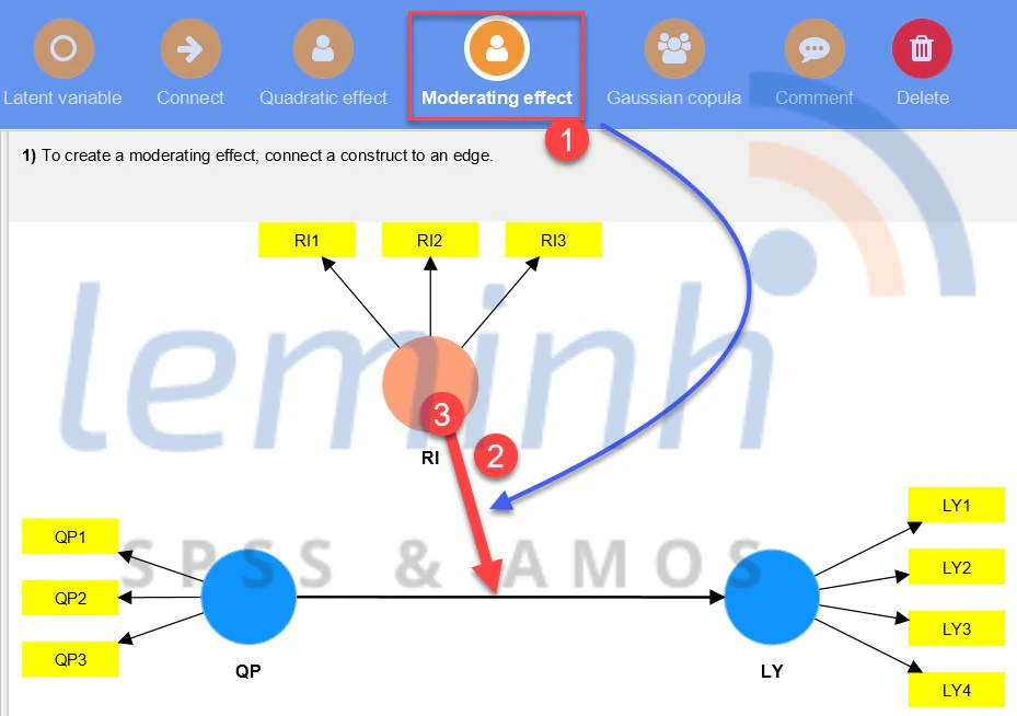
Add the moderation effect
Select the moderation tool and connect M to the X → Y path. Check the X × M interaction name and outcome variable Y.
Run the PLS-SEM Algorithm
Assess loadings or weights, reliability, AVE, HTMT, and VIF before interpreting the structural model.
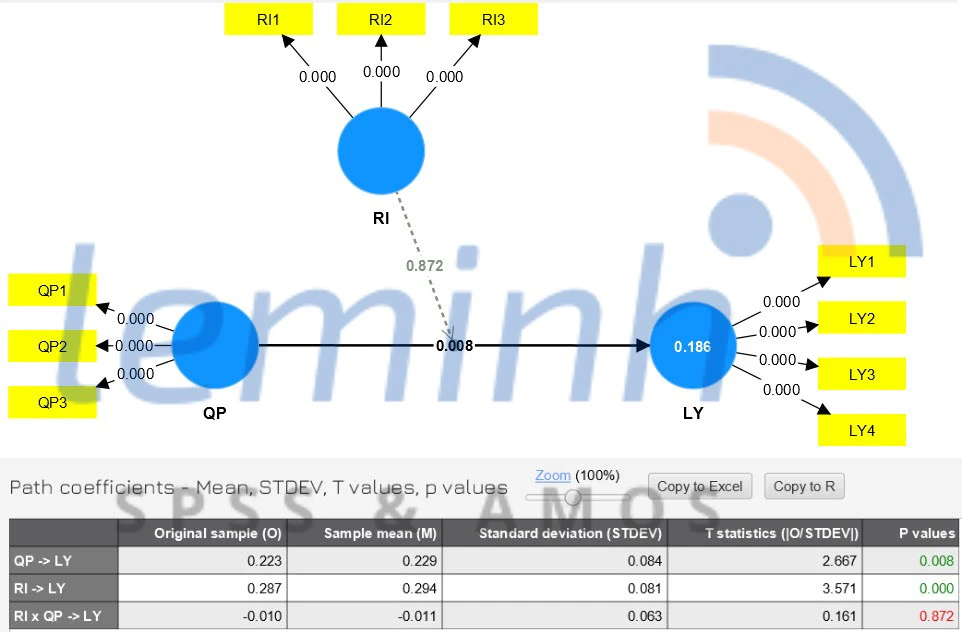
Run bootstrapping
Read the X × M → Y coefficient, standard error, t, p, and confidence interval. An interval containing 0 means there is insufficient evidence of an interaction at the chosen level.
Read the interaction’s f²
Assess the change in R² attributable to X × M. Interaction effects are often small, so do not dismiss a result solely because f² is low if theory and the confidence interval support it.
Open the simple slope plot
Interpret slopes at meaningful M values, commonly the mean and standard deviations. For binary M, read the two lines corresponding to groups 0 and 1.
Save tables and figures
Retain the coefficient table, confidence intervals, f², and simple slope plot so the report can be checked.
6. Numerical Example: From the Interaction Coefficient to Simple Slopes
This example only illustrates the calculation. Suppose X is Service Quality, M is standardized Switching Costs, and Y is Loyalty. The results give b₁ = 0,30 and b₃ = -0,12.
At M = -1 standard deviation, X’s conditional effect is 0,30 + (-0,12 × -1) = 0,42. At M = 0, the slope is 0,30. At M = +1 standard deviation, it falls to 0,18. The negative interaction coefficient indicates that higher Switching Costs weaken the relationship between Service Quality and Loyalty.
If b₃’s bootstrap confidence interval is [-0,20; -0,04], it excludes 0 and supports moderation. If the interval is [-0,25; 0,01], the negative point estimate alone is insufficient for a conclusion because the uncertainty still includes no interaction.
| M level | Formula | X → Y slope | Interpretation |
|---|---|---|---|
| Low (-1 SD) | 0,30 + (-0,12 × -1) | 0,42 | Strongest positive relationship |
| Average (0) | 0,30 + (-0,12 × 0) | 0,30 | Effect at average M |
| High (+1 SD) | 0,30 + (-0,12 × 1) | 0,18 | Weaker positive relationship |
A higher line merely indicates higher predicted Y values in that region. Moderation is identified by differences in slopes, not simply by vertical distances between lines.
7. Combining Coefficients, Confidence Intervals, f², and Plots
Begin with b₃ and its confidence interval. If there is evidence of an interaction, examine f² to describe its explanatory contribution, then use simple slopes to identify the direction of change. A p-value does not indicate whether the interaction is large or small, and simple slopes do not replace bootstrap testing.
When simple slope lines cross, the sign and magnitude of X → Y may change within the observed range. Descriptions at -1 SD, the mean, and +1 SD may then be insufficient. Examine the observed range carefully or use a region-of-significance technique if the software and research design permit (Dawson, 2014; Hayes and Rockwood, 2017).
| b₃ and confidence interval | Simple slope | Appropriate conclusion |
|---|---|---|
| Confidence interval excludes 0 | Slopes change in the hypothesized direction | Evidence supports the moderation hypothesis |
| Confidence interval excludes 0 | Slopes change opposite to the hypothesized direction | Moderation is present, but the directional hypothesis is unsupported |
| Confidence interval includes 0 | The plotted lines appear different | Insufficient statistical evidence of moderation |
| Very small but significant b₃ | Nearly parallel slopes | Explicitly describe the small effect and consider practical significance |
8. Common Errors and Corrections
| Weak practice or wording | Why it is incorrect | Correction |
|---|---|---|
| M has p < 0,05, so moderation is present | This is the direct effect b₂ | Test X × M → Y |
| The interaction is negative, so M harms Y | b₃ describes changes in the X → Y slope | Calculate conditional effects and interpret simple slopes |
| Divide continuous M into high and low groups | Information is lost and power is reduced | Keep M continuous unless theory requires groups |
| Code a binary variable as 1/2 | The value 0 does not identify the reference group | Use 0/1 coding and specify group 0 |
| Report only the p-value | Magnitude and uncertainty remain unknown | Report β, 95% CI, p, f², and the plot |
| Add interactions after examining the data | Increased risk of selective reporting | State hypotheses and theoretical justification before analysis |
9. APA 7 Reporting Template and Checklist
The following template uses the hypothetical values from the example. When substituting actual results, retain the variable names, reference group, standardization approach, and number of bootstrap samples used.
Example report
The moderating effect of Switching Costs on the relationship between Service Quality and Loyalty was estimated using the two-stage approach in SmartPLS 4. The interaction coefficient was negative, β = -.120, 95% bootstrap confidence interval [-.200, -.040], p = [value], f² = [value]. The conditional effect of Service Quality on Loyalty decreased from .420 at low Switching Costs (-1 SD) to .180 at high Switching Costs (+1 SD). These results support the hypothesis that Switching Costs weaken the relationship between Service Quality and Loyalty.
- Clearly identify X, M, Y, and the moderated path.
- Describe how M was coded or standardized.
- Report the number of bootstrap samples and confidence-interval type.
- Report the interaction’s β, 95% CI, p, and f².
- Present simple slopes numerically and graphically.
- Do not infer moderation from M’s direct effect.
- Distinguish continuous moderation from between-group MGA.
Conclusion
Moderation analysis addresses a conditional question: how does the effect of X on Y change as M changes? The interaction coefficient tests the change, while simple slopes show its direction and the levels at which it occurs.
A complete report connects four components: model specification, the bootstrap results for b₃, effect size, and the slope plot. Omitting any component makes the conclusion harder to verify or easier to misinterpret.
References
- Becker, J.-M., Ringle, C. M., & Sarstedt, M. (2018). Estimating moderating effects in PLS-SEM and PLSc-SEM: Interaction term generation and data treatment. Journal of Applied Structural Equation Modeling, 2(2), 1-21.https://doi.org/10.47263/JASEM.2(2)01
- Dawson, J. F. (2014). Moderation in management research: What, why, when, and how. Journal of Business and Psychology, 29(1), 1-19.https://doi.org/10.1007/s10869-013-9308-7
- Hayes, A. F., & Rockwood, N. J. (2017). Regression-based statistical mediation and moderation analysis in clinical research: Observations, recommendations, and implementation. Behaviour Research and Therapy, 98, 39-57.https://doi.org/10.1016/j.brat.2016.11.001
- Ringle, C. M., Wende, S., & Becker, J.-M. (2024). SmartPLS 4 [Computer software]. SmartPLS.https://www.smartpls.com
- SmartPLS. (n.d.). Moderation analysis in PLS-SEM: Two-stage approach.https://www.smartpls.com/documentation/algorithms-and-techniques/extended-relationships/moderation/
Academic note: The example values illustrate calculations rather than actual research results. Three-way moderation, moderated mediation, and nonlinear outcomes require their own specifications and interpretations.