
Second-Order Models in AMOS: Specification, Testing, and Competing Models
High correlations among first-order factors are insufficient grounds for a second-order factor. The model is meaningful only when a common concept explains covariances among dimensions and the specification is preferable to reasonable competing models.
The CB-SEM workflow starts with correlated first-order CFA, then specifies a second-order factor, checks identification, second-order loadings and disturbances, evaluates fit, compares first-order and bifactor models, and tests invariance for group comparisons. With exactly three first-order factors, the second-order layer may be just identified, so fit cannot independently confirm higher-order theory.
From lower-order components to a higher-order construct
- Theory
Define the role of each component
- Measurement
Assess lower-order constructs
- Higher order
Specify relationship directions
- Verification
Assess and report each stage
Conceptual diagram. Reflective or formative directions need conceptual justification.
Source: Lê Minh · Conceptual illustration, not software output.1. Learning objectives and prerequisites
After this guide, you should distinguish second-order factors from composites and bifactor models, draw the correct arrows in AMOS, recognize a just-identified second-order layer, interpret loadings alongside disturbances, compare competing models and report in APA 7 style.
Prerequisites are clearly defined first-order factors, sufficiently good indicators and an admissible correlated first-order CFA solution. Do not introduce a second-order factor to conceal weak first-order loadings, impossible correlations or unresolved discriminant validity.
- The second-order concept has a definition extending beyond each dimension.
- Each first-order factor has its own content domain.
- The first-order model has been assessed beforehand.
- There are no negative variances or impossible loadings.
- The number of first-order factors supports the testing objective.
- Competing models have been specified in advance.
2. What question does a second-order factor answer?
In a second-order factor model, indicators reflect first-order factors, while a second-order factor explains correlations among those factors. Marsh and Hocevar (1985) used CFA to investigate first-order and higher-order structures and their invariance across groups.
The second-order factor is a common factor, not an average score constructed from dimensions. Arrows point from the second-order factor to the first-order factors because the model assumes a common cause behind their covariances.
If dimensions jointly form an index and removing a dimension changes the concept's meaning, composite logic may be more appropriate. Conventional higher-order CFA in AMOS does not automatically address composite models; reversing arrows is insufficient to turn a factor model into a formative measurement model.
| Structure | Relationship to items or dimensions | Main question | Reason for caution |
|---|---|---|---|
| Second-order factor | A general factor explains first-order factors | Does a common cause explain covariances among dimensions? | High correlations without supporting theory |
| Composite | Dimensions combine to form the concept | How does the combination of components define the index? | Treating higher-order CFA as a composite model |
| Bifactor | Each item loads directly on a general and one specific factor | Do general and specific variance coexist at item level? | Calling a bifactor model a second-order model |
3. Correlated factors, second-order and bifactor models are not equivalent
A correlated first-order model allows dimensions to correlate freely. A second-order model explains those correlations through a higher-order factor, imposing structure on the first-order factor covariance matrix.
In a bifactor model, each item loads directly on a general factor and one specific factor, often specified as orthogonal factors. Reise (2012) explains that bifactor models separate general and specific variance at item level, rather than providing another notation for second-order CFA.
Brown (2015) and Kline (2023) recommend jointly considering theory, identification, parameter estimates, residuals and model comparisons. Selecting the best-fitting model while ignoring factor meaning may yield attractive but indefensible solutions.
In a second-order model, the general factor affects items through first-order factors. In a bifactor model, the general factor loads directly on each item.
4. Identification and the limitations of only three dimensions
Each first-order factor requires scaling, typically by fixing one loading to 1 or fixing its variance. The same logic applies to the second-order factor. Each first-order factor becomes endogenous at the second layer and requires a disturbance.
With exactly three first-order factors loading on one second-order factor, the second-order component is often just identified. The number of covariances among three factors equals the number of second-layer parameters after scaling, allowing the model to reproduce those covariances exactly.
Consequently, overall fit may equal that of the correlated first-order model. In that case, fit provides no strong test of the second-order structure. More weight must be placed on theory, second-order loadings, plausible disturbances, competing models and validation data.
| Situation | Consequence | Response |
|---|---|---|
| Two first-order factors | Usually insufficient information for a second-order factor | Do not specify a simple second-order factor |
| Three first-order factors | Second layer may be just identified | Do not use fit as the sole evidence |
| Four or more first-order factors | Degrees of freedom allow testing of the second-layer structure | Assess fit and residuals |
| Second-order loading near 1 | The dimension's disturbance may be very small | Check for Heywood cases and substantive distinctness |
| Negative disturbance | Improper solution | Stop and check the model and data |
5. Building a second-order model in AMOS
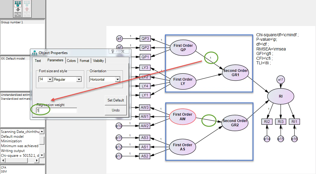
According to IBM Corp. (2022), AMOS allows direct diagram specification of factors, regression paths, variances and disturbances. Start from a validated correlated first-order CFA file and save a new version before adding the second-order factor.
Remove the two-headed covariances among first-order factors and replace them with one-headed paths from the second-order factor to each first-order factor. Add a disturbance to each first-order factor if AMOS has not created one. Retain item residuals.
Use the same data, estimator and missing-data treatment for model comparisons. If items, residual covariances and second-layer structure change simultaneously, the source of fit changes becomes unclear.
Estimate correlated first-order CFA
First check loadings, variances, factor correlations, residuals and fit.
Save a new model file
Retain the first-order model as a comparator and label versions clearly.
Create a second-order latent factor
Add an ellipse named for the general concept.
Draw paths to first-order factors
Arrows run from the second-order factor down to the first-order factors.
Remove first-order covariances
Do not retain all free covariances alongside second-order paths without a specific specification.
Add disturbances
Each endogenous first-order factor needs a second-layer error term.
Scale the second-order factor
Fix one loading to 1 or fix the variance using a consistent convention.
Estimate and read warnings
Check convergence, negative variances, out-of-range loadings and indefinite matrices.
Save standardized estimates and fit
Record second-order loadings, disturbances, first-order R-squared values and fit indices.
6. Assessing second-order loadings, disturbances and fit
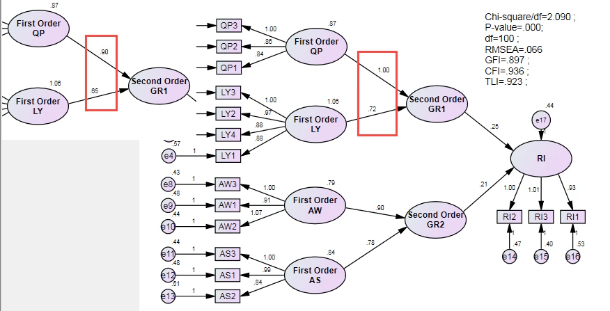
The standardized loading from the second-order factor to a first-order factor indicates how much of that dimension's variation the general factor explains. In a simple standardized specification, its square is the explained proportion of first-order factor variance.
A high loading does not make a dimension redundant. Each dimension must still contribute distinct content. A low loading may suggest that a dimension does not belong to the general construct, but removal requires definitions and validation, rather than a p-value alone.
Read the fit profile: chi-square, df, CFI, TLI, RMSEA with its confidence interval, SRMR where available, and residuals. Avoid a single cutoff. With a just-identified three-dimension second layer, fit matching the first-order model does not validate the HOC.
| Component | Meaning | Caution |
|---|---|---|
| Second-order loading | Association between the general factor and each dimension | Do not remove dimensions solely for falling below a loading threshold |
| Squared loading | Dimension variance explained by the HOC | Interpret only with an appropriate standardized solution |
| First-order disturbance | Dimension variance unexplained by the HOC | Negative values indicate an improper solution |
| Global fit | How well the model reproduces observed covariances | Does not independently confirm theory |
| Residuals | Locations of poor model reproduction | Do not add covariances mechanically |
7. Hypothetical numerical example: second-order service quality
The following scenario is illustrative, not real research data. Suppose Service Quality is a second-order factor comprising Reliability, Responsiveness, Assurance and Empathy. Each dimension has three items and correlated first-order CFA has produced an admissible solution.
The standardized second-order loadings are .82, .76, .71 and .68. Explained variances for the four dimensions are approximately .67, .58, .50 and .46. Model fit is chi-square = 148.6, df = 50, CFI = .951, TLI = .935, RMSEA = .069, 90% CI [.056, .082].
Empathy has the lowest loading but represents a distinct content domain. Do not remove it merely to raise the mean loading. The research team retains it and compares the second-order model against correlated first-order and substantively justified bifactor models.
| First-order factor | Loading | R-squared | Relative disturbance | Decision |
|---|---|---|---|---|
| Reliability | .82 | .67 | .33 | Retain |
| Responsiveness | .76 | .58 | .42 | Retain |
| Assurance | .71 | .50 | .50 | Retain |
| Empathy | .68 | .46 | .54 | Retain for content coverage |
8. Comparing competing models beyond fit alone
The correlated first-order model is the closest comparator because it permits dimension correlations without imposing a general factor. A second-order model is preferable when interdimension covariances fit a higher-order factor and the general concept is meaningful.
Bifactor models may fit better because they are more flexible, but can also produce weak specific factors or unstable solutions. Reise (2012) highlights restrictive bifactor assumptions and the need to examine both general and specific dimensions.
Compare models using the same items, sample and estimator. Appropriate chi-square difference tests can be used for nested models; for nonnested alternatives, consider fit, valid information criteria, parameter quality and interpretability. Kline (2023) emphasizes that good fit does not replace meaningful models.
| Model | Assumption | Strength | Risk |
|---|---|---|---|
| Correlated first-order | Dimensions correlate freely | Fewer restrictions on the source of covariance | No clear general score |
| Second-order | General factor explains interdimension covariance | Suited to hierarchical structure | May be just identified with three dimensions |
| Bifactor | General and specific factors load directly on items | Separates general and specific variance | Complexity and potentially weak specific factors |
9. Measurement invariance for second-order models
Comparisons of latent means or structural paths across groups require invariance assessment at both item and second-order levels. Chen, Sousa and West (2005) describe a sequence covering configural models, first-order loadings, second-order loadings, intercepts, disturbances and residual variances, depending on the objective.
Constraining only second-order loadings does not establish invariance. If item loadings or intercepts differ across groups, first-order factors may not share the same meaning or origin.
Partial invariance may be considered for unsupported constraints when justified and supported by sufficient anchor parameters. Disclose every released constraint rather than describing post-hoc selection as a confirmatory procedure.
Configural model
Maintain the same item, first-order and second-order factor structure across groups.
First-order loadings
Constrain item loadings to test first-layer metric invariance.
Second-order loadings
Constrain HOC-to-LOC relationships.
Observed intercepts
Check item origins for mean comparisons.
First-order intercepts
Assess the mean structure at dimension level.
Disturbances and residuals
Constrain only when stricter invariance is needed for the research question.
Compare latent means or paths
Proceed after establishing the required invariance and identify the reference group.
10. Common mistakes in second-order CFA
| Weak practice | Problem | Response |
|---|---|---|
| Creating an HOC because factors correlate highly | No substantive basis | Define the general construct first |
| Skipping first-order CFA | HOC conceals item and LOC problems | Validate the first layer first |
| Retaining free covariances among all LOCs | HOC no longer explains covariance as intended | Specify the source of associations clearly |
| Three LOCs and good fit imply a valid HOC | Second layer may be just identified | Also consider theory and alternatives |
| Calling bifactor second-order | Incorrect general-factor loading level | Draw and describe the models separately |
| Deleting low-loading LOCs | Narrows the content domain | Assess content and validate |
| Comparing groups without invariance testing | Differences may reflect measurement | Test invariance by layer |
11. APA 7 reporting template and checklist
The following template uses hypothetical values. In applications, also report the first-order comparator, scaling, estimator, missing-data treatment and every competing model.
Example reporting paragraph
Second-order CFA was estimated using IBM SPSS Amos [version], with [HOC] explaining four first-order factors: [list]. Each first-order factor was measured by [number] indicators and had its own disturbance. Standardized second-order loadings ranged from .68 to .82, corresponding to R-squared values of .46 to .67. Model fit was chi-square(50) = 148.60, CFI = .951, TLI = .935, RMSEA = .069, 90% CI [.056, .082], and SRMR = [ ]. Compared with correlated first-order and bifactor models, the second-order model was preferred because of [theory, parsimony and parameter quality]. Conclusions were limited by [sample size, design or invariance].
- Define the HOC and each LOC.
- Distinguish factors, composites and bifactor models.
- Validate correlated first-order CFA beforehand.
- Scale first-order and second-order factors.
- Give each first-order factor a disturbance.
- Check convergence and negative variances.
- Report second-order loadings with uncertainty.
- Read LOC R-squared values and disturbances.
- Report chi-square, df and the fit profile.
- Do not treat fit as the sole theoretical evidence.
- Retain the first-order model as a comparator.
- Compare justified competing models.
- Address the special case of only three LOCs.
- Check invariance before group comparisons.
- Match citations to the reference list.
Conclusion
Second-order CFA is useful when a general concept genuinely explains covariances among dimensions. It is not an automatic technique for combining highly correlated factors.
A defensible analysis demonstrates first-order quality, second-order identification, loadings, disturbances, fit, competing models and invariance where needed. With only three dimensions, theory and validation data become especially important because fit may not distinguish structures.
References
- Brown, T. A. (2015). Confirmatory factor analysis for applied research (2nd ed.). Guilford Press.https://www.guilford.com/books/Confirmatory-Factor-Analysis-for-Applied-Research/Timothy-Brown/9781462517794
- Chen, F. F., Sousa, K. H., & West, S. G. (2005). Testing measurement invariance of second-order factor models. Structural Equation Modeling, 12(3), 471-492.https://doi.org/10.1207/s15328007sem1203_7
- IBM Corp. (2022). IBM SPSS Amos 29 user's guide.https://www.ibm.com/docs/en/SSLVMB_29.0.0/pdf/IBM_SPSS_Amos_User_Guide.pdf
- Kline, R. B. (2023). Principles and practice of structural equation modeling (5th ed.). Guilford Press.https://www.guilford.com/books/Principles-and-Practice-of-Structural-Equation-Modeling/Rex-Kline/9781462551910
- Marsh, H. W., & Hocevar, D. (1985). Application of confirmatory factor analysis to the study of self-concept: First- and higher order factor models and their invariance across groups. Psychological Bulletin, 97(3), 562-582.https://doi.org/10.1037/0033-2909.97.3.562
- Reise, S. P. (2012). The rediscovery of bifactor measurement models. Multivariate Behavioral Research, 47(5), 667-696.https://doi.org/10.1080/00273171.2012.715555
Academic note: The example values were constructed to illustrate output interpretation. Second-order, bifactor and composite models answer different questions; do not select a model solely for fit or software convenience.