

MEANING OF THE COEFFICIENT R², f², Q², q² IN THE PLS SEM MODEL
- Determination coefficient R² or correction R²
R² or adjusted R² are coefficients that determine the extent to which an endogenous variable in an SEM model is explained by the exogenous variables related to it. For example:
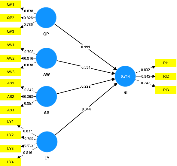
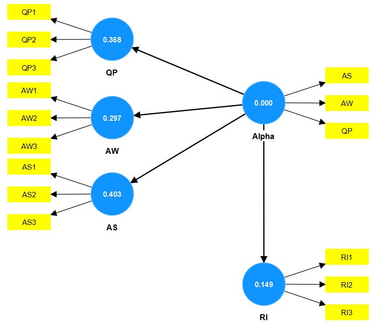
R² in the model above is 71.4%, this means that 71.4% of the variation in RI variable is adjusted by the 4 independent variables in the model (QP, AW, AS, LY). Percentage of change in RI variable adjusted by other factors not included in the research model. A research model is considered satisfactory when it has a large R² (for multiple regression models, the standard R² is ≥ 50%).
And to consider and evaluate the level of explanation of exogenous variables to endogenous variables in the model, the coefficient f² is used.
- The coefficient evaluates the degree of explanation of the exogenous variable to the endogenous variable f²
The coefficient f² is often considered together with the coefficient of determination R² to evaluate the degree of explanation of exogenous variables to endogenous variables in the model. This assessment aims to consider whether the explanatory role of exogenous variables on endogenous variables exists or not? And if so, is the level low or high? Normally, people often use the f² index to consider selecting variables with a high level of explanation to focus resources on improving these factors in the research model.
| Assess the degree of explanation of the exogenous variable on the endogenous variable using the coefficient f² | |
| f² < 0.02 | Does not play an explanatory role |
| 0.02 ≤ f2 < 0.15 | Has a low level of explanation |
| 0.15 ≤ f2 < 0.35 | Has a medium level of explanation |
| f2 ≥ 0.35 | Has a high level of explanation |
In conventional multiple regression models, we use SPSS for analysis and few people mention the coefficient f², but only focus on the regression coefficient in the model. People often rely on the regression coefficient (beta) to evaluate the influence of independent variables on the dependent variable. And from there, it serves as a basis for selecting factors that need to focus resources to improve in the research model. However, this needs to be considered carefully, because a cause and effect relationship in a model with a high regression coefficient does not necessarily mean that the coefficient f² is high. Let’s compare the analytical results from the actual model in the table below.
| Regression coefficient (beta) | Coefficient f² | |
| AS → RI | 0.222 | 0.110 |
| AW → RI | 0.334 | 0.273 |
| LY → RI | 0.344 | 0.264 |
| QP → RI | 0.191 | 0.088 |
To make it easier to visualize, let’s visualize it graphically as follows:
We can see that the order from largest to smallest of the independent variables in the model according to the beta regression coefficient is LY, AW, AS, QP. However, the order from largest to smallest according to the coefficient f² will be AW, LY, AS, QP. So if a business’s resources are limited, and it is necessary to choose only one best factor to improve, then we should consider carefully.
- Coefficient to evaluate the accuracy of Q2 forecast
Q2 is an index of out-of-sample predictive power in the model. To calculate this Q2 coefficient, in SmartPLS 4 software, select Calculate, click Blindfolding, leave everything as default and click Start calculation.

To read the results, click on Construct cross-validated redundancy. Note that, the Q2 factor is calculated by SmartPLS using two different methods. One is the cross-validated redundancy approach, and the other is the cross-validated communality approach. Therefore, the results report screen will appear with 2 results corresponding to the 2 approaches above. Any result we use is ok. However, according to many documents, the cross-validated redundancy approach gives better results. Therefore, we also recommend that you use the results from this approach.
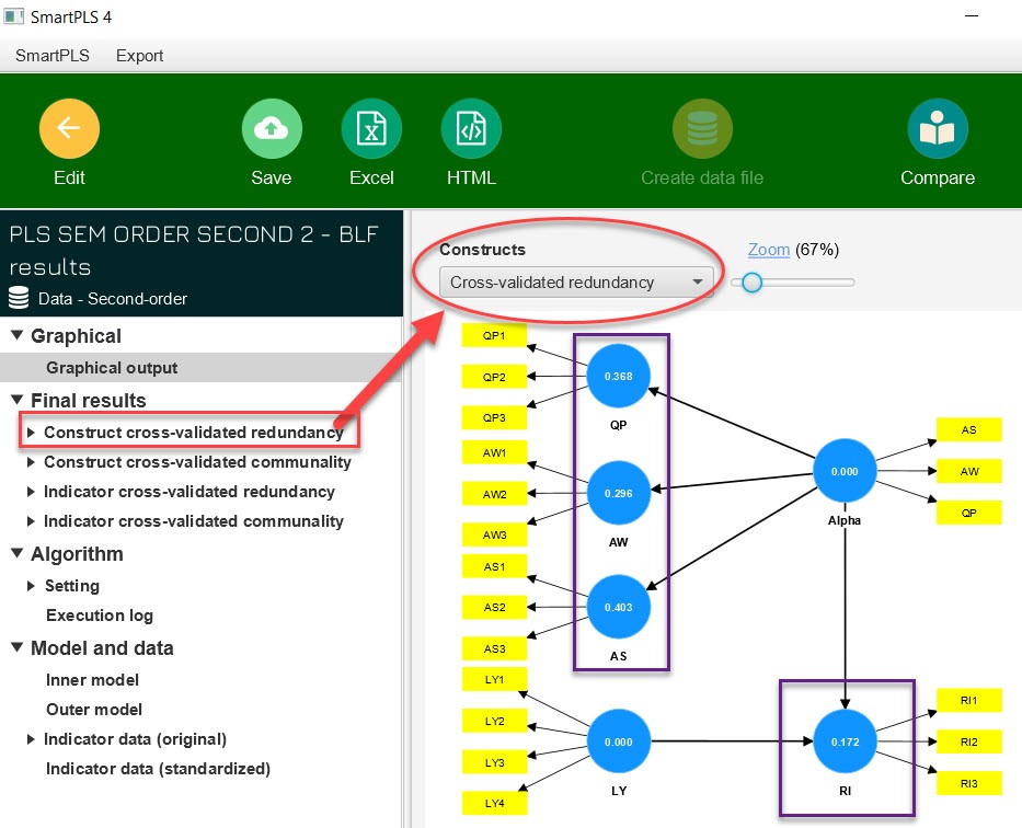
In the right pane of the screen, we see the model with Q2 coefficients located inside the circles (construct variables) corresponding to the approach, we can choose the approach for the model to represent the corresponding Q2 coefficient. Another thing to note is that the Q2 coefficient only appears with endogenous variables, with purely exogenous variables the Q2 coefficient will not appear.
Results in the analysis example in the figure: the RI factor has Q2 = 0.172, meaning that the forecasting accuracy of the RI structure (out-of-sample forecasting capacity) is 17.2% ≤ 25%, so according to Vu Huu Thanh and Nguyen Minh Ha (2023), the RI variable measurement model has a low level of prediction accuracy. Below are Q2 evaluation standard frameworks cited from Vu Huu Thanh and Nguyen Minh Ha (2023).
| Evaluate the level of forecast accuracy | |
| 0 < Q2 ≤ 0.25 | Short |
| 0.25 < Q2 ≤ 0.5 | Medium |
| Q2 > 0.5 | High |
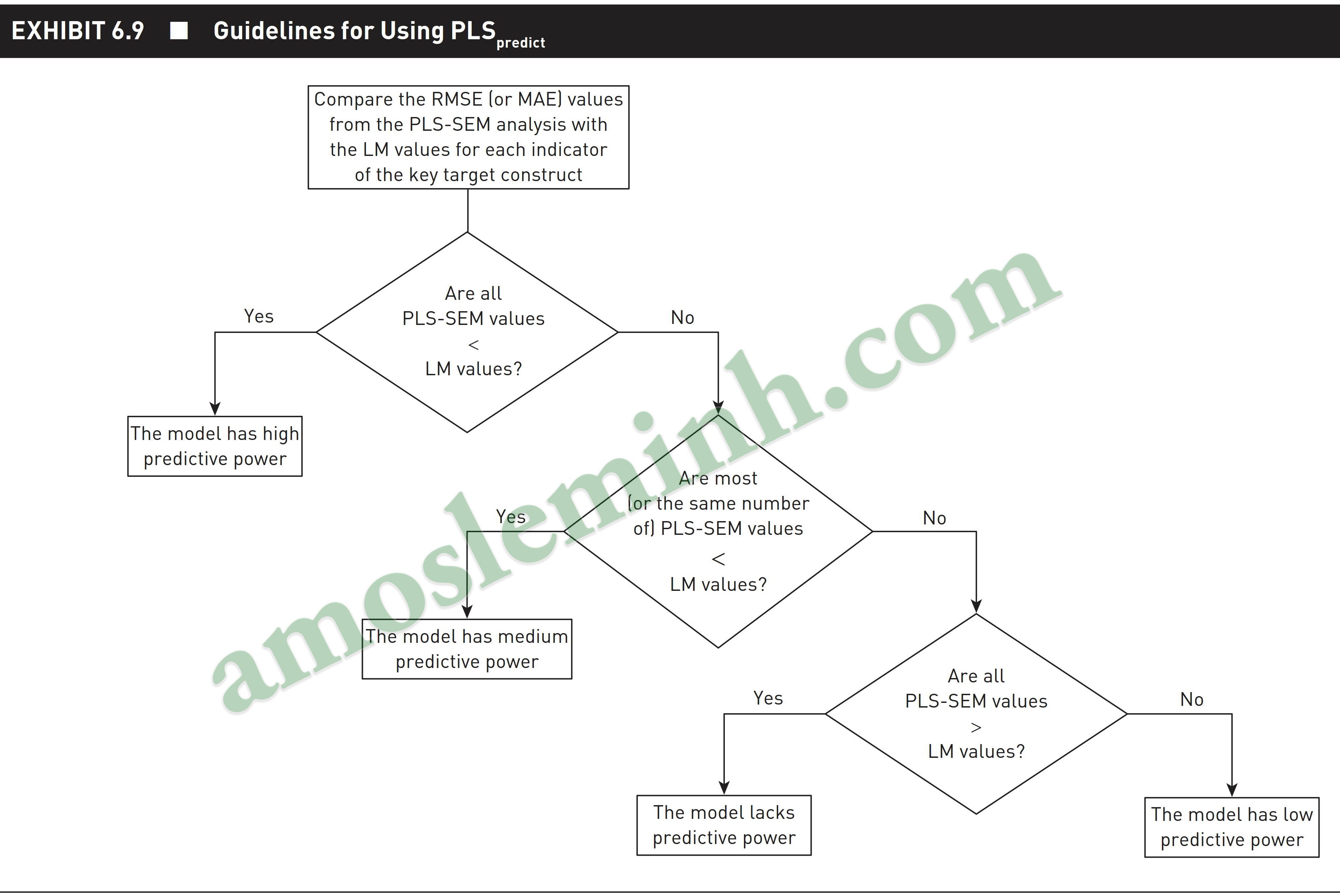
Above is a way to evaluate the level of forecasting according to the Q2 coefficient that is commonly used in previous studies. However, as Hair et al (2022) argue, the Q2 coefficient does not actually evaluate the model’s predictive ability (Exhibit 6.6). Therefore, Hair et al (2022) presented a PLS prediction procedure (PLSpredict). This procedure compares the results of the RMSE (the root mean square error – measures the model’s average error from the actual data) value or the MAE (mean absolute error – MAE also measures the average error) value. model compared to the actual data, however MAE calculates the average of the absolute value of the error) between the PLS model and the LM model (linear regression model benchmark). The process for evaluating the model’s predictive capacity is given by Hair and colleagues (2022) as follows (we quote verbatim from the author):
Next, we will show you how to evaluate the model’s prediction level using the PLSpredict procedure in SmartPLS 4.
Step 1: Select the PLSpredict procedure. Leave it as default and run analysis.
Step 2: Read the results. You select MV prediction summary. You can use column number 1 (RMSE) or column number 2 (MAE). Combined with Table Exhibit 6.9 of Hair et al. (2022) to conclude about the model’s predictive capacity. The example results show that the RI model’s predictive capacity is high, the remaining models do not have predictive capacity.
- Coefficient to evaluate the predictive effectiveness of an explanatory variable q2
This coefficient is used when you evaluate the model’s predictive capacity using the Q² coefficient. In case you evaluate the model’s predictive capacity using the PLSpredict procedure then there is no need to evaluate the q2 coefficient, we only need to evaluate R2 and f2 (refer to Hair et al., 2022).
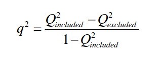
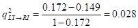
The coefficient evaluating the predictive effectiveness of an explanatory variable q2 also known as the impact coefficient q2. Q2 of the RI variable is 0.172 ≤ 0.25 → the level of forecasting accuracy is low. We need to consider that RI is explained by two variables, Alpha and LY, so which of these two variables has a higher predictive effect for RI? And specifically, how is the level of forecast assessed? We need to consider the coefficient q2, which is calculated using the following formula:
In there:
• Q2included is the Q2 coefficient of the original model
• Q2excluded is the coefficient Q2 of the model that has eliminated the latent variable that needs to be evaluated q2
| RI | |
| Alpha | q2 = ? |
| LY | q2 = ? |
Alpha variable type model:
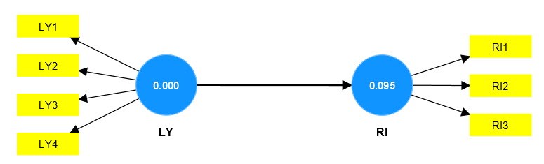
LY variable type model:

| RI | |
| Alpha | 0.093 → Forecasting efficiency is low |
| LY | 0.028 → Forecasting efficiency is low |
Below are the q2 assessment standards frameworks cited from Vu Huu Thanh and Nguyen Minh Ha (2023).
| Evaluate the predictive effectiveness of an explanatory variable | |
| q2 < 0.02 | There is no predictive effect |
| 0.02 ≤ q2 < 0.15 | Low forecasting efficiency |
| 0.15 ≤ q2 < 0.35 | Average forecasting performance |
| q2 ≥ 0.35 | High forecasting efficiency |
References
Hair, J., & Alamer, A. (2022). Partial Least Squares Structural Equation Modeling (PLS-SEM) in second language and education research: Guidelines using an applied example. Research Methods in Applied Linguistics, 1(3), 100027.
Vu Huu Thanh, & Nguyen Minh Ha. (2023). Data analysis textbook applying the PLS – SEM model (1st ed.). Ho Chi Minh City National University Publishing House.