T-TEST AND ONE-WAY ANOVA ANALYSIS GUIDE
(PART 1 – BASICS)
To have the best and most practical knowledge about basic statistical methods, we personally recommend that you read the book series by Hoang Trong and Chu Nguyen Mong Ngoc published in 2008. We rate that this set of books (including 2 basic and advanced volumes) is the most condensed and concise knowledge to date. Please limit your reference to knowledge online. Whatever research you do, you need to have scientific sources to be convincing.
I. BASIC THEORY
T-Test and One-Way ANOVA are two common statistical methods used to test differences between groups of data. Here’s a quick breakdown of both of these methods:
- T-Test (T-Test):
T-Test is a statistical method used to test whether there is a meaningful difference between two groups of data. The T-Test evaluates the difference between the means of two groups and determines whether this difference can be considered statistically significant.
There are two main types of T-Test:
- Independent T-Test: Use when we want to compare the average of a variable between two independent groups (not dependent on each other).
- Paired T-Test: Use when we want to compare the average of a variable in the same group in two different times.
→ The purpose of T-Test is to test whether the difference between means is large enough to be considered statistically significant.
When running the T-test, compare it with the following table to conclude (Hoang Trong and Chau Nguyen Mong Ngoc, 2008):
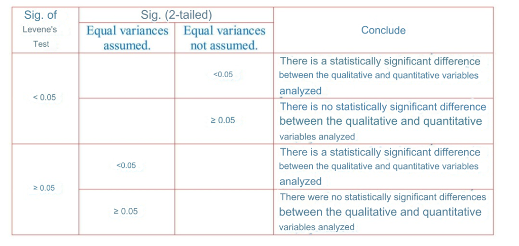
Note that T-test only performs pairwise comparisons. So for variables that need to be tested for differences that have more than 2 groups, we have to do it pair by pair. This will take time, and the accuracy of the results will no longer ensure 95% reliability. Therefore, in this case, we will turn to the One-way ANOVA test. This test will help us compare groups at the same time.
- One-Way ANOVA (One-Way Analysis of Variance):
One-Way ANOVA is a statistical method used to test differences between three or more groups of data. It evaluates whether there is a meaningful difference between the means of groups of data.
One-Way ANOVA assumes that the groups of data being tested are normally distributed and have equal variances. If the results of the analysis show a meaningful difference between at least two of the groups, we can perform further analyzes to determine which group contains the difference.
→ The purpose of One-Way ANOVA is to examine the differences between the means of three or more groups to determine whether at least one group is significantly different from the other groups.
In both T-Test and One-Way ANOVA, the ultimate goal is to evaluate the differences between groups of data and determine whether these differences are statistically significant. Note that, before performing any analysis, we need to check the assumptions of data distribution and variance, to ensure the validity and reliability of the analysis results. To evaluate the normal distribution of data, you can see more in our older article here. In this article, we assume that the data ensures normal distribution.
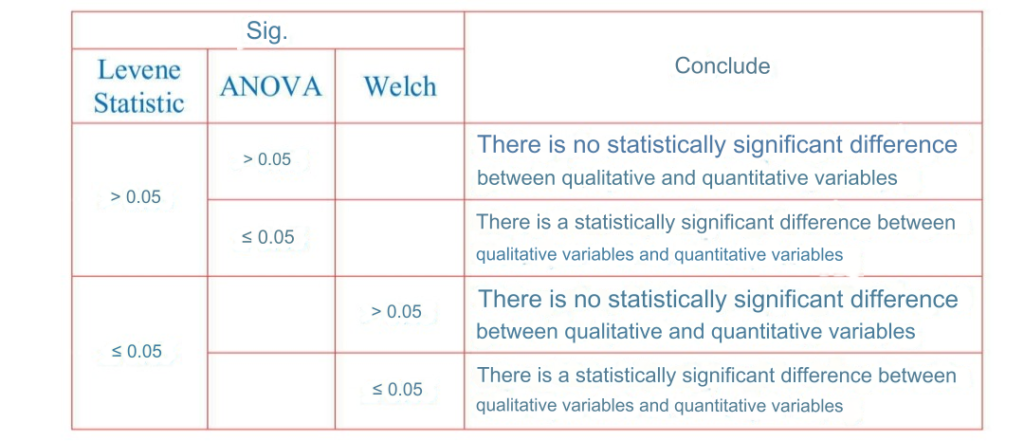
When running the One-Way ANOVA test, you need to compare with the following table to conclude (Hoang Trong and Chu Nguyen Mong Ngoc, 2008; Salcedo & McCormick, 2023):
II. ANALYSIS PRACTICE
Next, we will conduct sample T-test and One-way ANOVA analysis. Our dependent variable is RI (Repeat Purchase Intention), and demographic variables include: Purchase Group, Gender, Age and Education Level. Characteristics of Demographic variables as Table below.
Note that, within the scope of this article, we will not go into detail about how to run analysis using SPSS software. If you are interested, you can read the documents shared by Le Minh Data Service. here.
| Variable name | Encode | Characteristic |
| Buying group | 1 | The group buys at the traditional market |
| 2 | The group buys at convenience stores or supermarkets | |
| Gender | 1 | Male |
| 2 | Female | |
| Age | 1 | ≤ 22 year old |
| 2 | 23 to 30 years old | |
| 3 | 31 to 45 year old | |
| 4 | Over 45 years old | |
| Academic level | 1 | ≤ high school |
| 2 | Intermediate college | |
| 3 | University | |
| 4 | After university |
We note that T-test is only performed for variables with 2 groups or less. For variables with 3 groups or more, One way Anova test needs to be run. In this example case, we run T-test for the variables Buying Group and Gender, the remaining variables Age and Education level will be run One way Anova test. Here, we only present the sample run for the variables Purchasing Group and Education Level.
- Group buying
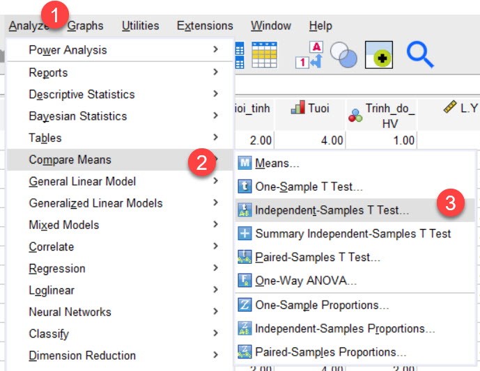
To run a T-test for the Buying Group, we perform the steps as shown below.
Then read the results.
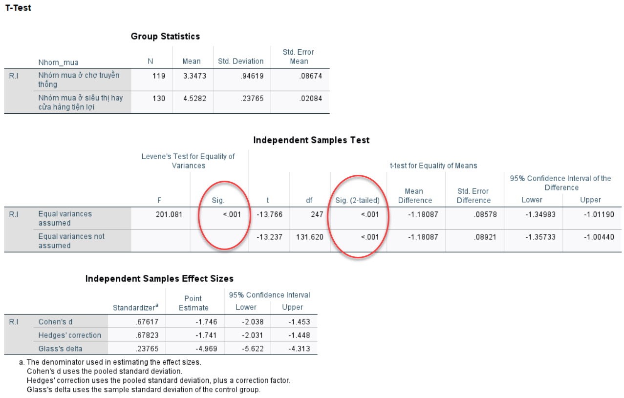
Sig values. all reached statistical significance (≤ 5%), so it can be concluded that the purchasing group has a statistically significant difference in customers’ repeat purchase intention. To further evaluate the repeat purchase intention of the two buying groups (which group has higher repeat purchase intention) without running MGA, we do the following. We copy the Group Statistics table into Excel, then draw a graph of the MEAN value as shown below. Later, I will present in detail how to calculate this Mean value. We temporarily understand this mean value as the mean value of the dependent variable RI corresponding to each buying group.
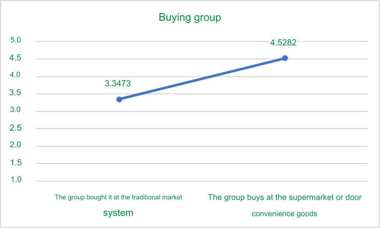
From the graph, it can be seen that the group that buys at supermarkets or convenience stores has a higher tendency to repeat purchase of the product than the group that buys at traditional markets.
- Education level
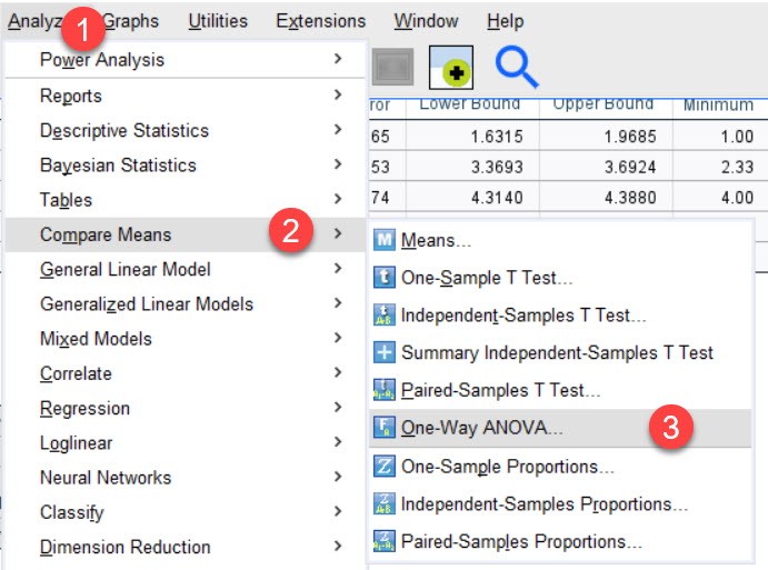
For Educational Level, we will perform One way Anova test. The steps are implemented as shown below.
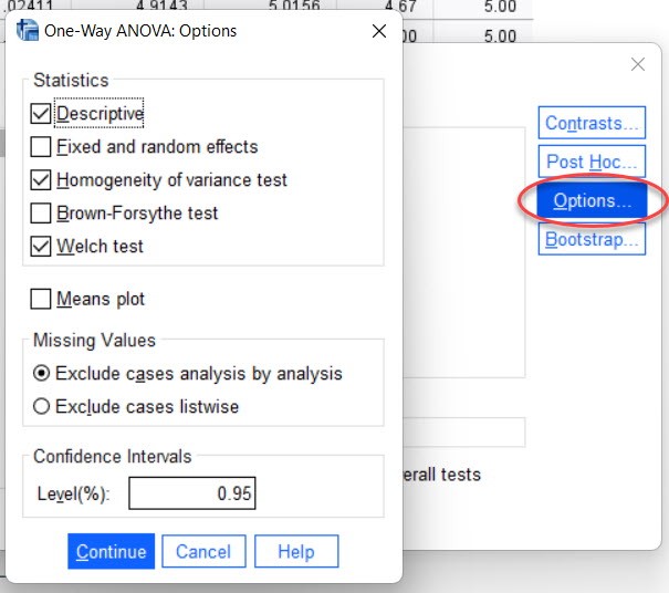
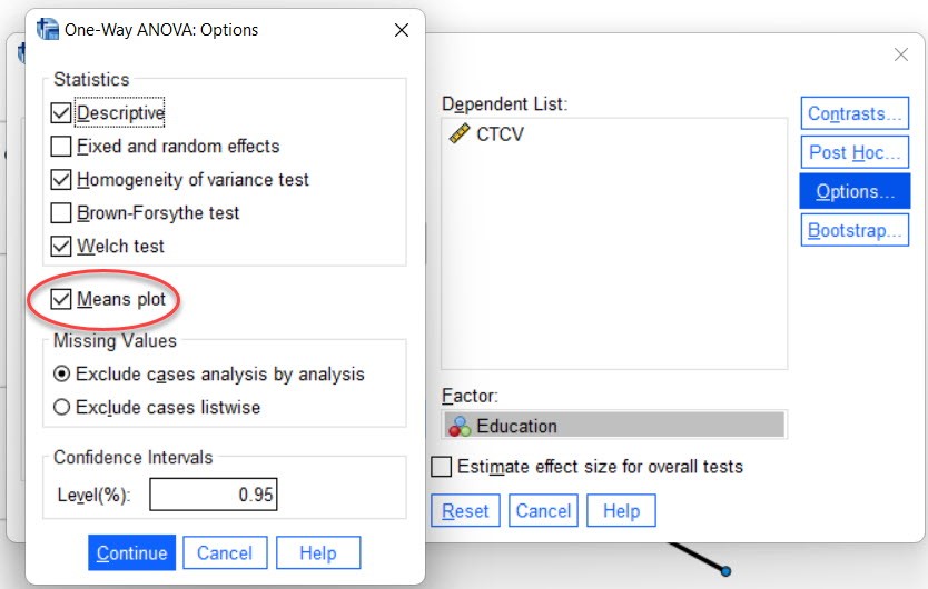
Ở phần option chúng ta lựa chọn như hình, các mục khác cứ để mặc định nhé.
Read the results
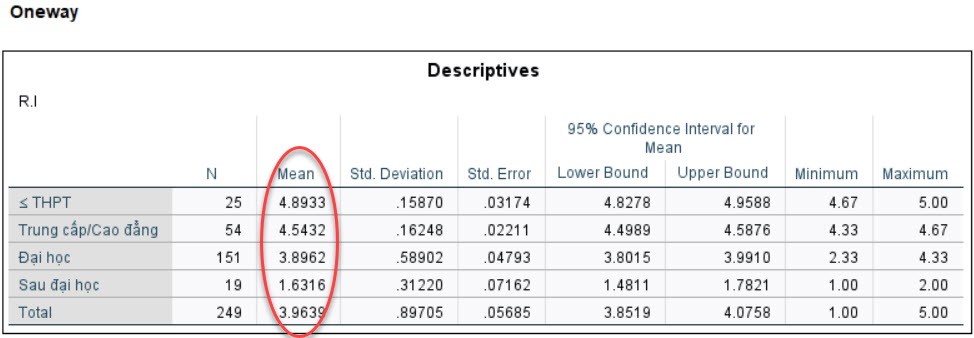
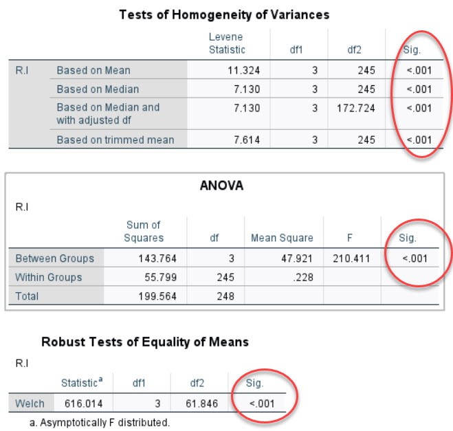
Sig values. all reached statistical significance (≤ 5%), so it can be concluded that education level has a statistically significant difference with customers’ intention to repeat purchase of the product. Specifically, we conduct additional graphical analysis of the mean value as follows. You can also copy the group statistics table into Excel and draw a graph for the mean value.
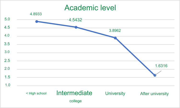
Looking at the graph, we can see that the lower the level, the more likely people are to repeat purchases.
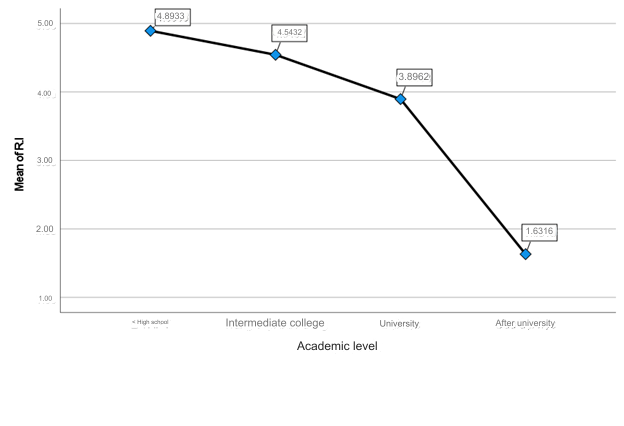
If we don’t want to show the graph in Excel for easy viewing, we can use the SPSS tool to graph the mean value. To draw a graph when choosing T-test or Anova analysis, remember to click and select Means plot as shown below.
The graph results are drawn directly in SPSS as follows:
III. General comments and how to calculate the mean value in the Group Statistics table
For T-test and One-way Anova analysis, we can only make a preliminary assessment and the trend of the groups of variables with respect to the variables we compare. To further analyze how each group of variables affects the research model, we need to conduct in-depth analyzes such as MGA.
Now we will learn how the program calculates the mean value in the statistical table.
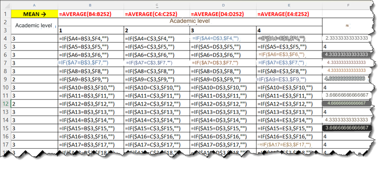
The mean value in the statistical table of variable groups is the mean value of the comparison object variable (here the RI variable – Repeat purchase intention) according to each variable group. For example, I will calculate the mean value for One way Anova analysis of the variable Education Level. First, we copy the Education Level variable column and the RI variable into the excel file.
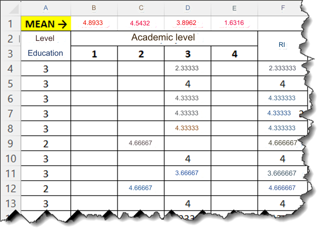
The formula I use in Excel is as follows: We just install the formula as in cell B4 and then drag and drop it to finish.
So here we have temporarily finished guiding you to analyze T-test and One way Anova tests. If you have any need for data, please contact Le Minh Data Service. Sincerely thank you.
For some basic explanations for T-test and Anova One-way, we would like to quote verbatim from George, D., & Mallery, P. (2021).
_1-20230807145641.jpg)
References
George, D., & Mallery, P. (2022). IBM SPSS statistics 27 step by step: A simple guide and reference. Routledge. https://doi.org/10.4324/9781003205333
Hoang Trong and Chu Nguyen Mong Ngoc. (2008). Analyze research data with SPSS. Hong Duc Publishing House.
Salcedo, J., & McCormick, K. (2023). SPSS statistics for dummies. John Wiley & Sons.


