

ASSESSING NORMALITY OF DATA USING SPSS AMOS
(ASSESSMENT OF NORMAL DISTRIBUTION OF DATA)
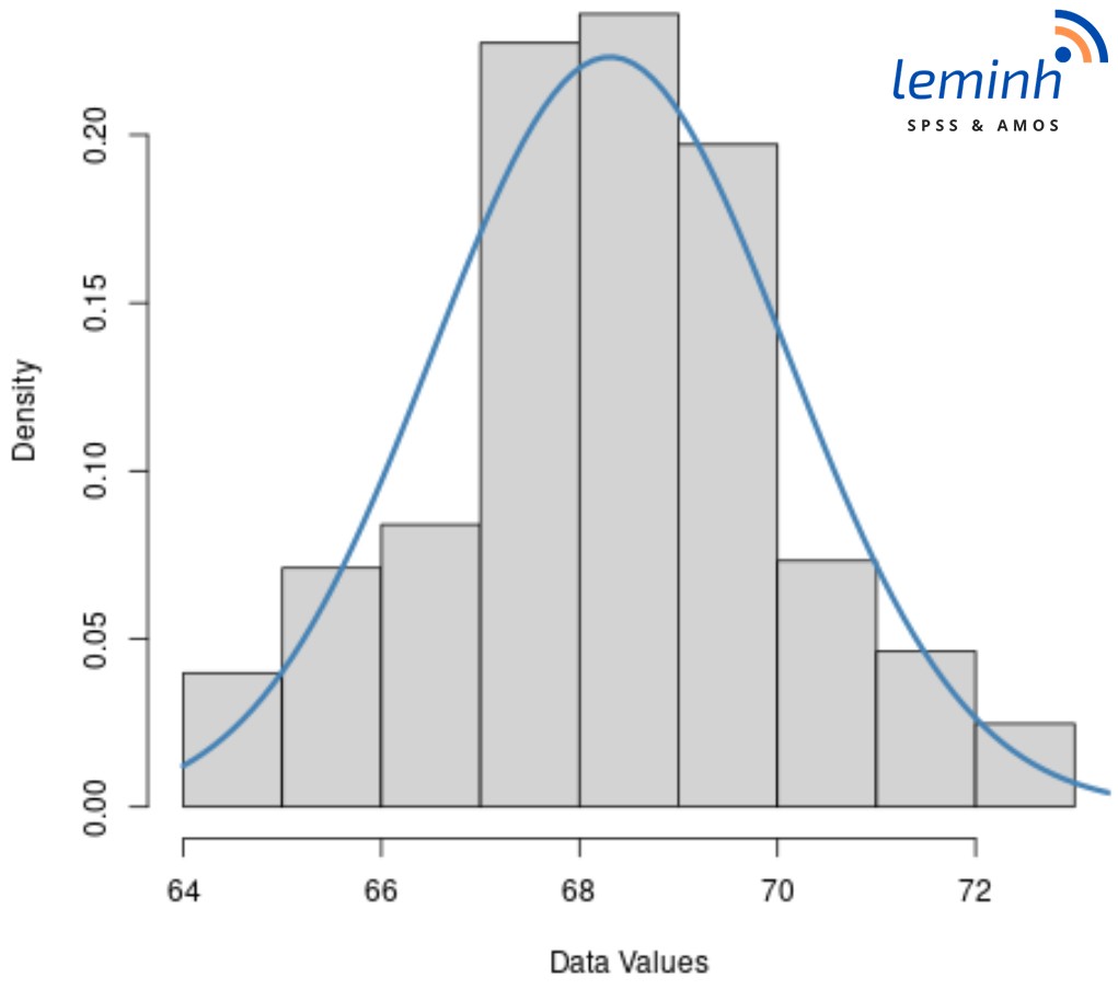
In this article, we will learn techniques for checking the validity of data. The normal distribution is a continuous probability distribution that is symmetric around its mean, most observations cluster around a central peak, and the probability for values far from the mean decreases with both direction. The standard normal distribution is a normal distribution with a mean (μ) of 0 and a standard deviation (σ) of 1. The normal distribution is also called a bell curve because the graph of the probability density has a bell shape.
Testing the normal distribution is an important step in the inferential statistical procedure, helping us basically determine the general shape of a distribution, thereby evaluating whether the test is skewed or not, and whether there is a skew. positive or negative. Normal distribution test is used to check whether a set of data follows a normal distribution or not. If the data set follows a normal distribution, we can use statistics related to normal distribution such as t-test and ANOVA. In addition, other statistics are also performed such as: average value (mean); standard deviation; percentile; Pearson correlation coefficient; Test a hypothesis about the mean value of a sample (t-test). If the data does not follow a normal distribution, we can use other methods such as the Mann-Whitney U or Kruskal-Wallis test. However, these methods have the disadvantage of being insensitive to outliers and do not allow the use of statistics related to normal distribution.
Normally, to identify a normal distribution in SPSS, you can use the following methods:
- View a chart with a standard curve (Histograms with normal curve) with a symmetrical bell shape with the highest frequency in the middle and gradually lower frequencies on both sides.
- Draw a normal probability plot (normal Q-Q plot) – normal distribution when the graph has a linear relationship (straight line).
- Check Skewness and Kurtosis values of the independent variable. If Skewness and Kurtosis are between -1 and 1, the distribution of the independent variable is considered normal distribution (Hair et al., 2019, p.48). According to Collier (2020), the Skewness range is between -2 and 2, and the Kurtosis range is between -10 and 10, then the data is considered to be normally distributed. If your data does not have a normal distribution, using the maximum likelihood estimation method is not possible, but must be replaced with another estimation method such as GLM – general linear model (Collier, 2020, p.166).
Next we use SPSS to test the normal distribution for the data set.
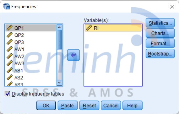
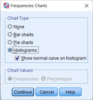
First, at the main interface of SPSS, click on Analyze > Descriptive Statistics > Frequencies… Put the variables that need to be tested into the Variable(s) box. Continue clicking the commands in the order Charts > Histograms > Show normal curve on histogram. Click Continue > OK and wait for the results.
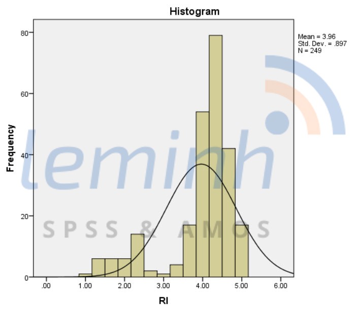
Draw a standard curve chart:
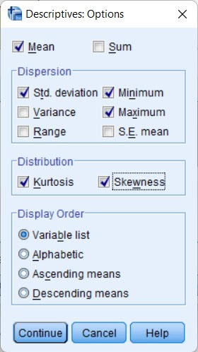
On the toolbar, click Analyze > Descriptive Statistics > Descriptives. Put the variable to be tested into the Variable(s) box, click Options. Check the Kurtosis and Skewness boxes, select Continue and click OK, then wait for the results.
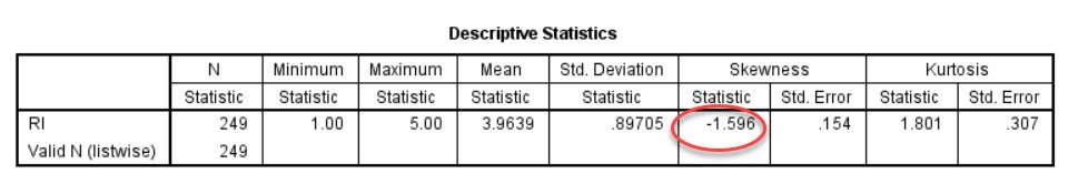
The Skewness value of the independent variable is -1.596, then it can be concluded that the distribution of the independent variable is not a normal distribution. However, to draw more accurate conclusions about the normality of the distribution, you can use other tests such as the Shapiro-Wilk or Kolmogorov-Smirnov test.
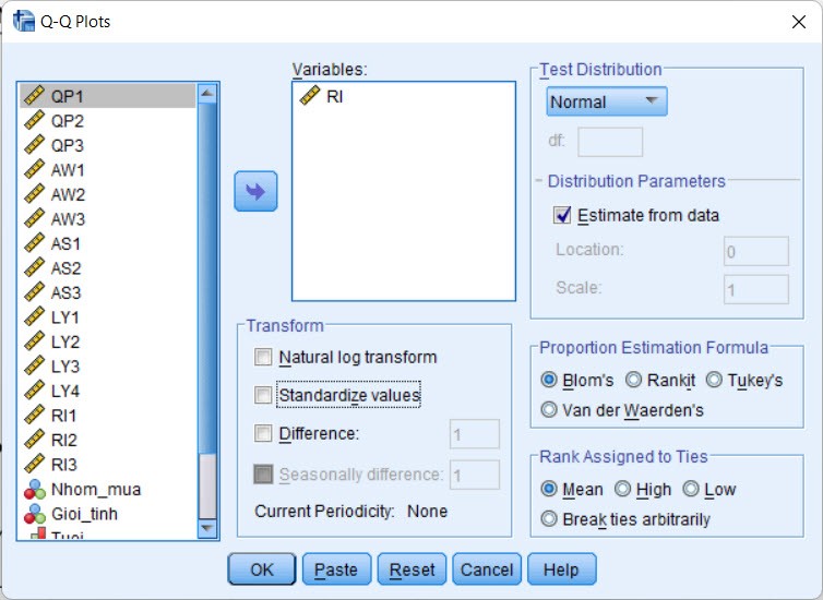
Draw a standard probability chart (Q-Q chart)
The Q-Q plot shows a visualization of the distribution of data, often used with studies with large sample sizes (>100). How to draw a Q-Q graph is as follows.
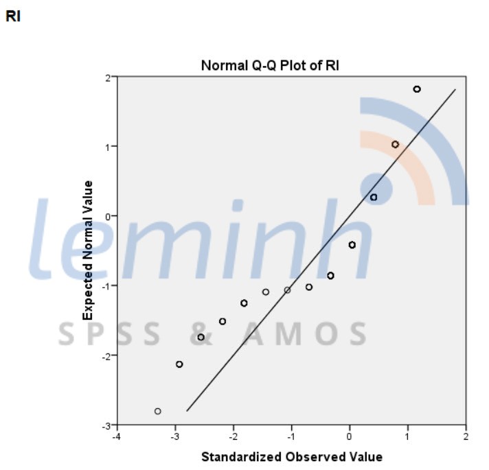
It can be seen that the dots are distributed far away from the trend line. This provides further evidence that the data are not normally distributed. We can completely combine this Q-Q chart with the results of the above statistical tests to confirm for sure whether this data is normally distributed or not.
Normality Assessment
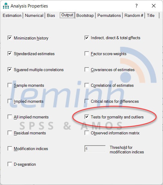
In AMOS to evaluate the normal distribution of data, we use the Tests for normality and outliers technique.
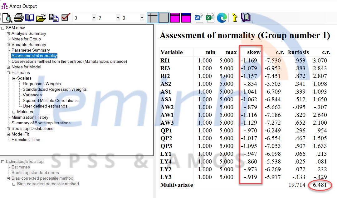
If the absolute value of skewness is ≤ 1, the data is considered to be normally distributed. However, SEM uses an MLE (Maximum Likelihood Estimator) Tool like AMOS that is quite powerful with skewness having an absolute value greater than 1.0 if the sample size is large and the Critical Region (CR) for skewness does not exceed 8.0. This means, we can conduct a deeper analysis (SEM) because the estimator used is MLE. Typically, sample sizes greater than 200 are considered large enough in MLE even though the data distribution is not normal. For kurtosis, the range is −10 to +10 then the data is still considered normally distributed (Collier, 2020).
There are many ways to handle data such as removing items with large deviations. However, the most popular recent method is to continue the analysis with MLE (without deleting any items and without discarding any observations) and reconfirm the results of the analysis through Bootstrapping. Bootstrapping is the process of resampling on an existing data set using the sampling with replacement method. The statistical procedure calculates the mean and standard deviation for each sample of size N to produce a new sampling distribution.
References:
Collier, J. E. (2020). Applied structural equation modeling using AMOS: Basic to advanced techniques. Routledge.
Hair, J. F., Anderson, R. E., Tatham, R. L., & Black, W. C. (2019). Multivariate Data Analysis. In Cengage Learning (8th ed.). Cengage Learning.